Forecasting Healthy Ride Ridership With Prophet
This post is about predicting demand for the Healthy Ride bike system in Pittsburgh. I wanted to try out Facebook’s prophet package and try to do some time series forecasting.
As usual, load the required packages and set up the environment:
library(tidyverse)
library(lubridate)
library(prophet)
library(janitor)
library(hrbrthemes)

options(scipen = 999)

theme_set(theme_bw())
This code loads the data and formats the date column so the prophet package can interface with it. I use dir() to find all the CSV files in the folder and then set_names() and map_df(read_csv()) to read each of the CSV files into memory.
files <- dir("data", ".csv")

data <- str_c("data/", files) %>%
  set_names() %>%
  map_df(read_csv) %>%
  clean_names()

df <- data %>%
  filter(date < "2019-08-01") %>%
  count(date)

# df %>%
#   ggplot(aes(date, n)) +
#   geom_point()
#
# last(df$date)
The data I will use contains the number of rides per day and also includes the month and year. prophet will identify the time series patterns (“seasonality”) in the data and identify the “true” pattern
prophet has a plug-and-play workflow that is easy to use, but it has more stringent requirements for how the data has to be shaped. The date data has to be named ds and the target variable has to be named y. I set the floor to zero because there cannot be fewer than 0 rides in a day. prophet requires a cap
max_rides <- df %>%
  summarize(max_rides = max(n) * 3) %>%
  pull()

df <- df %>%
  mutate(n = log(n),
         cap = log(max_rides)) %>%
  filter(!is.na(date)) %>%
  rename(ds = date,
         y = n) %>%
  mutate(floor = 0)


df %>%
  filter(is.na(ds))
## # A tibble: 0 x 4
## # … with 4 variables: ds <date>, y <dbl>, cap <dbl>, floor <dbl>glimpse(df)## Rows: 1,518
## Columns: 4
## $ ds <date> 2015-05-31, 2015-06-01, 2015-06-02, 2015-06-03, 2015-06-04, 20…
## $ y <dbl> 6.173786, 4.844187, 4.934474, 4.875197, 5.361292, 5.609472, 5.9…
## $ cap <dbl> 8.013343, 8.013343, 8.013343, 8.013343, 8.013343, 8.013343, 8.0…
## $ floor <dbl> 0, 0, 0, 0, 0, 0, 0, 0, 0, 0, 0, 0, 0, 0, 0, 0, 0, 0, 0, 0, 0, …This creates the set of holidays I use in the model.
us_holidays <- prophet::generated_holidays %>%
  as_tibble() %>%
  filter(country == "US") %>%
  mutate(ds = as.Date(ds))
This code fits a model to the dataset.
m <- prophet(df, growth = 'logistic', holidays = us_holidays)make_future_dataframe() creates the dataframe that prophet uses to make its forecast. In this case, I have it create a dataframe with 365 days of additional rows to predict onto.
future <- make_future_dataframe(m, periods = 365, freq = "day") %>%
  mutate(floor = 0,
         cap = unique(df$cap))
This code performs the forecast on the future dataset.
forecast <- predict(m, future) %>%
  as_tibble()
The output is a dataframe with the date, the predicted ridership, and the upper and lower bounds of the prediction.
forecast## # A tibble: 1,883 x 66
## ds trend cap floor additive_terms additive_terms_…
## <dttm> <dbl> <dbl> <dbl> <dbl> <dbl>
## 1 2015-05-31 00:00:00 5.14 8.01 0 0.720 0.720
## 2 2015-06-01 00:00:00 5.14 8.01 0 0.657 0.657
## 3 2015-06-02 00:00:00 5.14 8.01 0 0.724 0.724
## 4 2015-06-03 00:00:00 5.14 8.01 0 0.765 0.765
## 5 2015-06-04 00:00:00 5.14 8.01 0 0.733 0.733
## 6 2015-06-05 00:00:00 5.14 8.01 0 0.784 0.784
## 7 2015-06-06 00:00:00 5.14 8.01 0 0.844 0.844
## 8 2015-06-07 00:00:00 5.14 8.01 0 0.754 0.754
## 9 2015-06-08 00:00:00 5.14 8.01 0 0.690 0.690
## 10 2015-06-09 00:00:00 5.14 8.01 0 0.755 0.755
## # … with 1,873 more rows, and 60 more variables: additive_terms_upper <dbl>,
## # `Christmas Day` <dbl>, `Christmas Day_lower` <dbl>, `Christmas
## # Day_upper` <dbl>, `Christmas Day (Observed)` <dbl>, `Christmas Day
## # (Observed)_lower` <dbl>, `Christmas Day (Observed)_upper` <dbl>, `Columbus
## # Day` <dbl>, `Columbus Day_lower` <dbl>, `Columbus Day_upper` <dbl>,
## # holidays <dbl>, holidays_lower <dbl>, holidays_upper <dbl>, `Independence
## # Day` <dbl>, `Independence Day_lower` <dbl>, `Independence Day_upper` <dbl>,
## # `Independence Day (Observed)` <dbl>, `Independence Day
## # (Observed)_lower` <dbl>, `Independence Day (Observed)_upper` <dbl>, `Labor
## # Day` <dbl>, `Labor Day_lower` <dbl>, `Labor Day_upper` <dbl>, `Martin
## # Luther King, Jr. Day` <dbl>, `Martin Luther King, Jr. Day_lower` <dbl>,
## # `Martin Luther King, Jr. Day_upper` <dbl>, `Memorial Day` <dbl>, `Memorial
## # Day_lower` <dbl>, `Memorial Day_upper` <dbl>, `New Year's Day` <dbl>, `New
## # Year's Day_lower` <dbl>, `New Year's Day_upper` <dbl>, `New Year's Day
## # (Observed)` <dbl>, `New Year's Day (Observed)_lower` <dbl>, `New Year's Day
## # (Observed)_upper` <dbl>, Thanksgiving <dbl>, Thanksgiving_lower <dbl>,
## # Thanksgiving_upper <dbl>, `Veterans Day` <dbl>, `Veterans Day_lower` <dbl>,
## # `Veterans Day_upper` <dbl>, `Veterans Day (Observed)` <dbl>, `Veterans Day
## # (Observed)_lower` <dbl>, `Veterans Day (Observed)_upper` <dbl>,
## # `Washington's Birthday` <dbl>, `Washington's Birthday_lower` <dbl>,
## # `Washington's Birthday_upper` <dbl>, weekly <dbl>, weekly_lower <dbl>,
## # weekly_upper <dbl>, yearly <dbl>, yearly_lower <dbl>, yearly_upper <dbl>,
## # multiplicative_terms <dbl>, multiplicative_terms_lower <dbl>,
## # multiplicative_terms_upper <dbl>, yhat_lower <dbl>, yhat_upper <dbl>,
## # trend_lower <dbl>, trend_upper <dbl>, yhat <dbl>plot automatically plots the forecast data:
plot(m, forecast)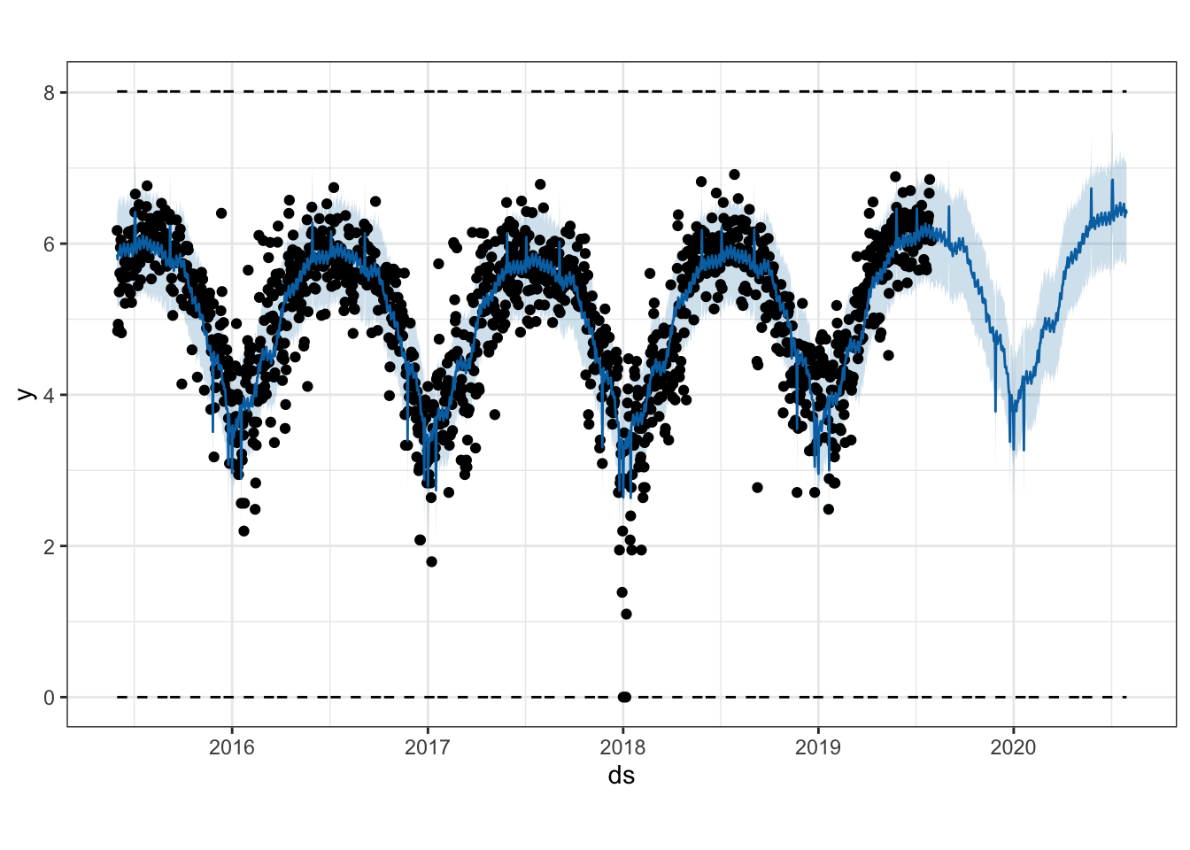
prophet also decomposes the various seasonal effects.
prophet_plot_components(m, forecast)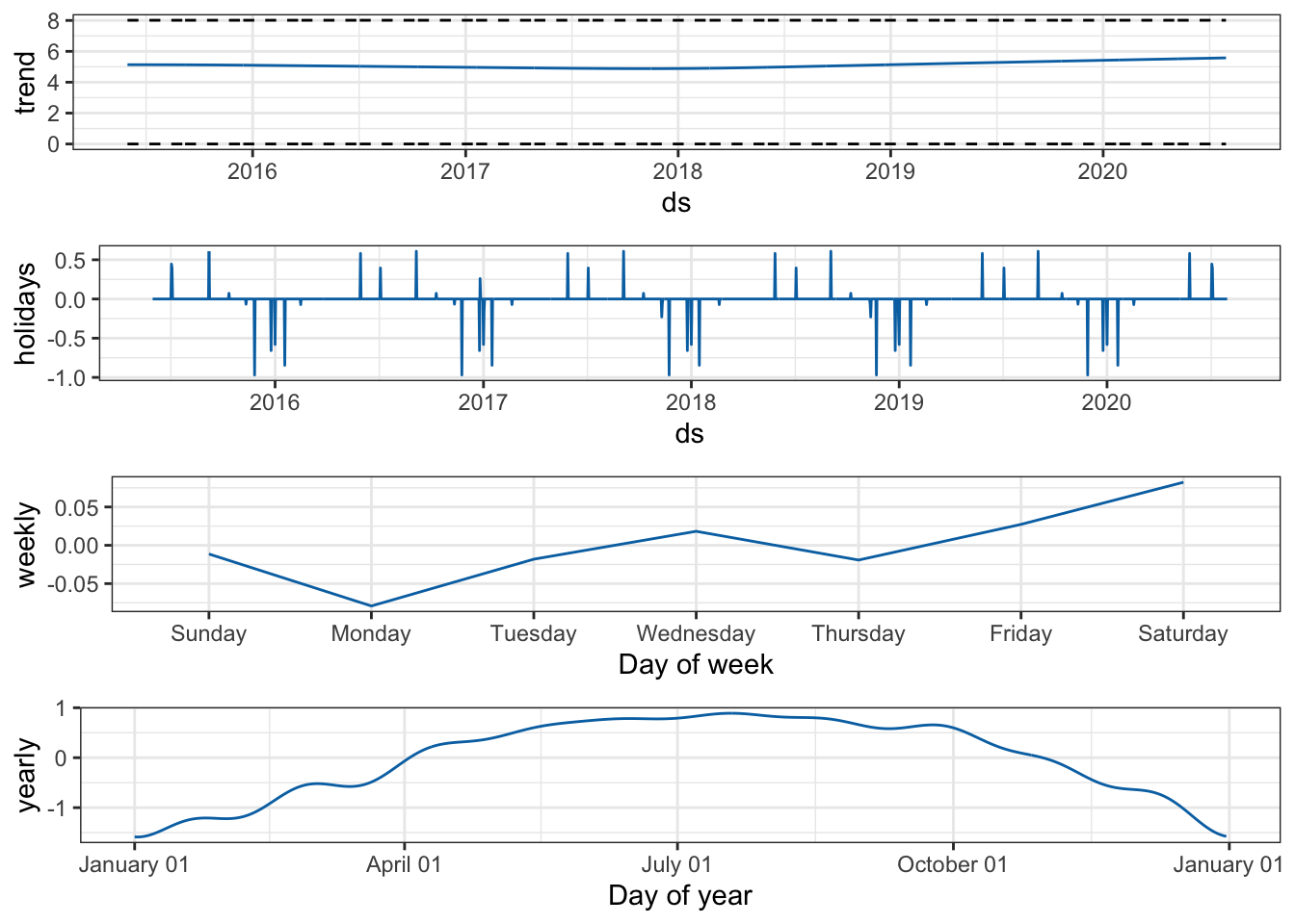
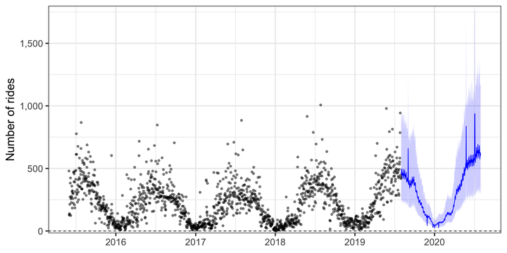
We can of course use ggplot to manually plot the data.
df_aug <- forecast %>%
  mutate(ds = ymd(ds)) %>%
  left_join(df) %>%
  mutate(yhat = exp(yhat),
         yhat_lower = exp(yhat_lower),
         yhat_upper = exp(yhat_upper),
         y = exp(y))

df_aug %>%
  ggplot(aes(x = ds)) +
    geom_ribbon(data = df_aug %>% filter(ds > last(df$ds)),
                aes(ymin = yhat_lower, ymax = yhat_upper), alpha = .2, fill = "blue") +
    geom_line(data = df_aug %>% filter(ds > last(df$ds)),
              aes(y = yhat), color = "blue") +
    geom_point(aes(y = y), alpha = .5) +
    geom_hline(aes(yintercept = unique(floor)), linetype = 2) +
    labs(x = NULL,
         y = "Number of rides") +
    scale_y_comma() +
  theme_bw(base_size = 20)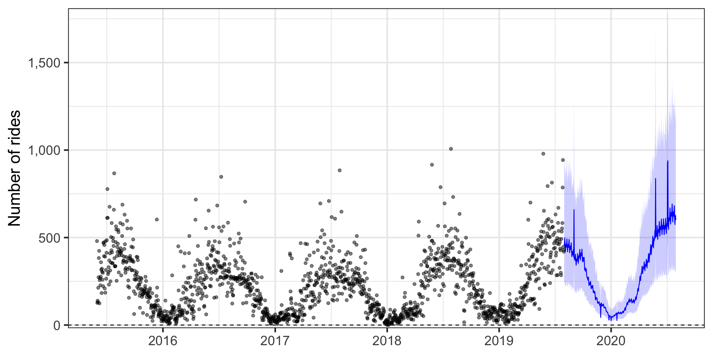
prophet also provides functions for cross-validation.
df_cv <- cross_validation(m, horizon = 30, units = 'days')

performance_metrics(df_cv) %>%
  as_tibble() %>%
  gather(metric, measure, -horizon) %>%
  ggplot(aes(horizon, measure)) +
  geom_line() +
  facet_wrap(~metric, scales = "free_y",
             ncol = 1) +
  labs(x = "Horizon",
       y = "Measure") +
  theme_bw()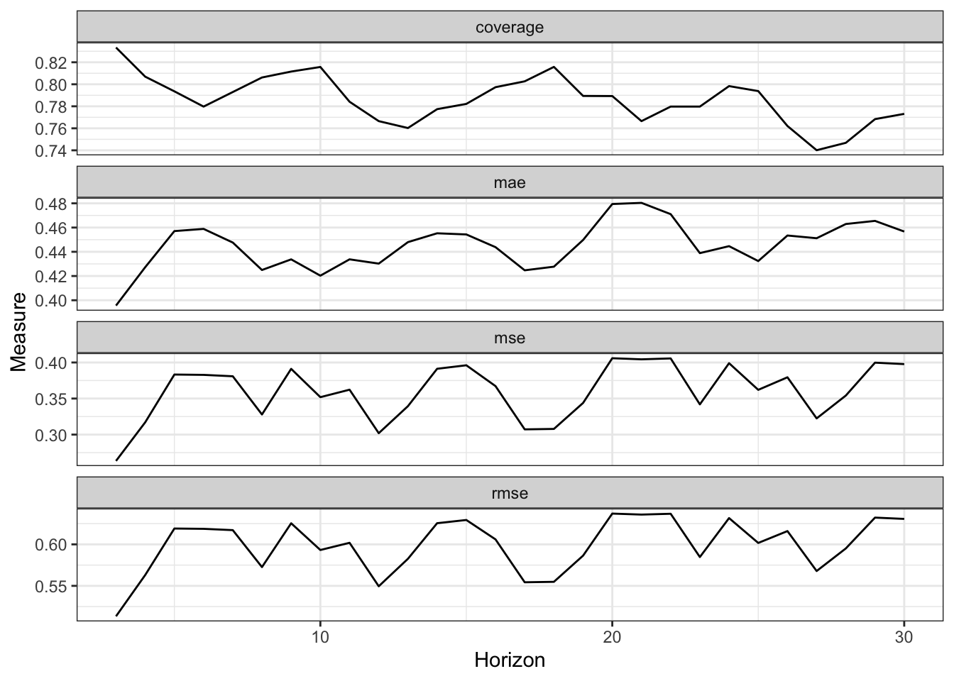
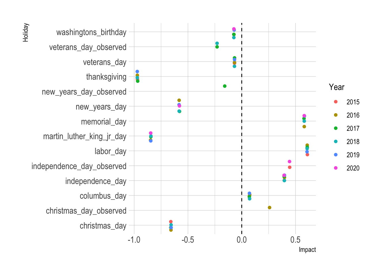
We can also inspect the impact of holidays on the prediction.
df_holiday_impact <- forecast %>%
  clean_names() %>%
  select(ds, christmas_day:washingtons_birthday) %>%
  select(-contains("upper"), -contains("lower")) %>%
  pivot_longer(-ds, names_to = "holiday", values_to = "value") %>%
  mutate(year = as.factor(year(ds))) %>%
  filter(holiday != "holidays",
         value != 0)

df_holiday_impact %>%
  arrange(ds) %>%
  mutate(holiday = as.factor(holiday)) %>%
  ggplot(aes(holiday, value, color = year)) +
  geom_hline(yintercept = 0, linetype = 2) +
  geom_jitter() +
  coord_flip() +
  labs(x = "Holiday",
       y = "Impact") +
  scale_color_discrete("Year") +
  theme_ipsum()