Effect of Geographic Resolution on ebirdst Abundance
While exploring some of the citizen science bird observation data available through ebirdst, I was confused by how to understand the calculation of ebirdst’s abundance metric.
The ebirdst documentation (?ebirdst::load_raster) defines abundance as:
the expected relative abundance, computed as the product of the probability of occurrence and the count conditional on occurrence, of the species on an eBird Traveling Count by a skilled eBirder starting at the optimal time of day with the optimal search duration and distance that maximizes detection of that species in a region.
I had seen some weird results when trying to manually calculate abundance as occurrence * count. My initial attempt had aggregated the results by month.
The underlying problem is that abundance and count are the results of models, and are subject to model error. I also believe that the data outputted from load_raster lacks the necessary significant digits to accurately recreate abundance. Lowering the resolution or aggregating the data will exacerbate this issue.
This code loads my convenience function to retrieve a metric for a species at a given geographic resolution. This gets occurrence, count, and abundance for the Northern Cardinal at high (3 km), medium (9 km), and low resolutions (27 km). The function also crops the underlying raster data to Allegheny County, PA.
library(here)
library(hrbrthemes)
library(patchwork)

source("https://raw.githubusercontent.com/conorotompkins/ebird_shiny_app/main/scripts/functions/pull_species_metric.R")

theme_set(theme_ipsum())

species_table <- crossing(species = c("Northern Cardinal"),
                          metric = c("occurrence", "count", "abundance"),
                          resolution = c("hr", "mr", "lr"))

species_table
## # A tibble: 9 × 3
## species metric resolution
## <chr> <chr> <chr>
## 1 Northern Cardinal abundance hr
## 2 Northern Cardinal abundance lr
## 3 Northern Cardinal abundance mr
## 4 Northern Cardinal count hr
## 5 Northern Cardinal count lr
## 6 Northern Cardinal count mr
## 7 Northern Cardinal occurrence hr
## 8 Northern Cardinal occurrence lr
## 9 Northern Cardinal occurrence mrspecies_metrics <- species_table %>%
mutate(data = pmap(list(species, metric, resolution), ~get_species_metric(..1, ..2, ..3))) %>%
mutate(resolution = fct_relevel(resolution, c("hr", "mr", "lr"))) %>%
arrange(species, metric, resolution)## 0.482 sec elapsed
## 18.461 sec elapsed
## 3.693 sec elapsed
## 0.336 sec elapsed
## 11.979 sec elapsed
## 0.086 sec elapsed
## 0.42 sec elapsed
## 13.353 sec elapsed
## 0.357 sec elapsed
## 0.365 sec elapsed
## 18.478 sec elapsed
## 3.375 sec elapsed
## 0.184 sec elapsed
## 12.043 sec elapsed
## 0.06 sec elapsed
## 0.4 sec elapsed
## 13.45 sec elapsed
## 0.356 sec elapsed
## 0.166 sec elapsed
## 18.944 sec elapsed
## 3.253 sec elapsed
## 0.284 sec elapsed
## 12.844 sec elapsed
## 0.054 sec elapsed
## 0.527 sec elapsed
## 14.384 sec elapsed
## 0.359 sec elapsedspecies_metrics## # A tibble: 9 × 4
## species metric resolution data
## <chr> <chr> <fct> <list>
## 1 Northern Cardinal abundance hr <tibble [1,813,448 × 7]>
## 2 Northern Cardinal abundance mr <tibble [221,312 × 7]>
## 3 Northern Cardinal abundance lr <tibble [25,012 × 7]>
## 4 Northern Cardinal count hr <tibble [1,813,448 × 7]>
## 5 Northern Cardinal count mr <tibble [221,312 × 7]>
## 6 Northern Cardinal count lr <tibble [25,012 × 7]>
## 7 Northern Cardinal occurrence hr <tibble [1,813,448 × 7]>
## 8 Northern Cardinal occurrence mr <tibble [221,312 × 7]>
## 9 Northern Cardinal occurrence lr <tibble [25,012 × 7]>This unnests the data and recalculates abundance (abundance_test) and the difference between actual abundance and abundance_test.
species_table_unnested <- species_metrics %>%
  unnest(data) %>%
  select(species, resolution, date, month, x, y, metric_desc, value) %>%
  pivot_wider(id_cols = c(species, resolution, date, month, x, y),
              names_from = metric_desc,
              values_from = value) %>%
  select(species, resolution, date, month, x, y, count, occurrence, abundance) %>%
  mutate(abundance_test = count * occurrence,
         diff = abundance - abundance_test)
Grouping by month to get to the county level changes the grain of the data so much that abundance_test undershoots abundance by 20%. This occurs at all resolutions.
species_metrics %>%
  unnest(data) %>%
  select(species, resolution, date, month, x, y, metric_desc, value) %>%
  pivot_wider(id_cols = c(species, resolution, date, month, x, y),
              names_from = metric_desc,
              values_from = value) %>%
  select(species, resolution, date, month, x, y, count, occurrence, abundance) %>%
  group_by(species, month, resolution) %>%
  summarize(occurrence = mean(occurrence, na.rm = T),
            count = mean(count, na.rm = T),
            abundance = mean(abundance, na.rm = T)) %>%
  ungroup() %>%
  mutate(abundance_test = count * occurrence,
         diff = abundance - abundance_test) %>%
  ggplot(aes(abundance, abundance_test)) +
  geom_abline() +
  geom_point() +
  facet_wrap(~resolution) +
  tune::coord_obs_pred()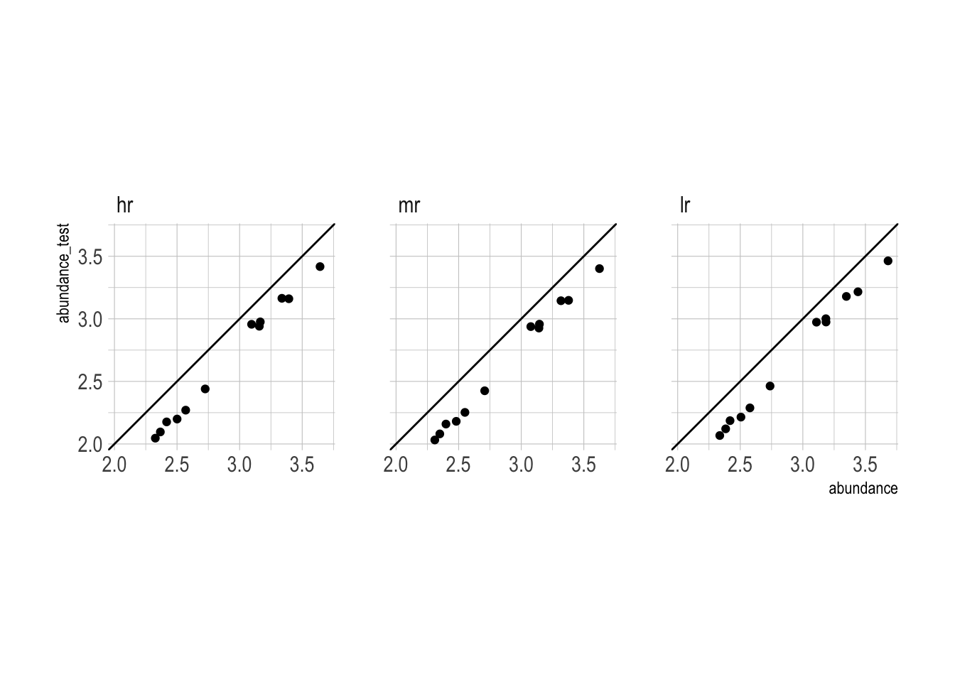
Totally un-aggregated, abundance_test closely resembles abundance, but degrades as resolution decreases.
species_table_unnested %>%
  select(abundance, abundance_test, resolution) %>%
  drop_na() %>%
  ggplot(aes(abundance, abundance_test)) +
  geom_density_2d_filled(contour_var = "ndensity") +
  facet_wrap(~resolution) +
  tune::coord_obs_pred() +
  coord_cartesian(xlim = c(0, 8),
                  ylim = c(0, 8)) +
  guides(fill = guide_colorsteps())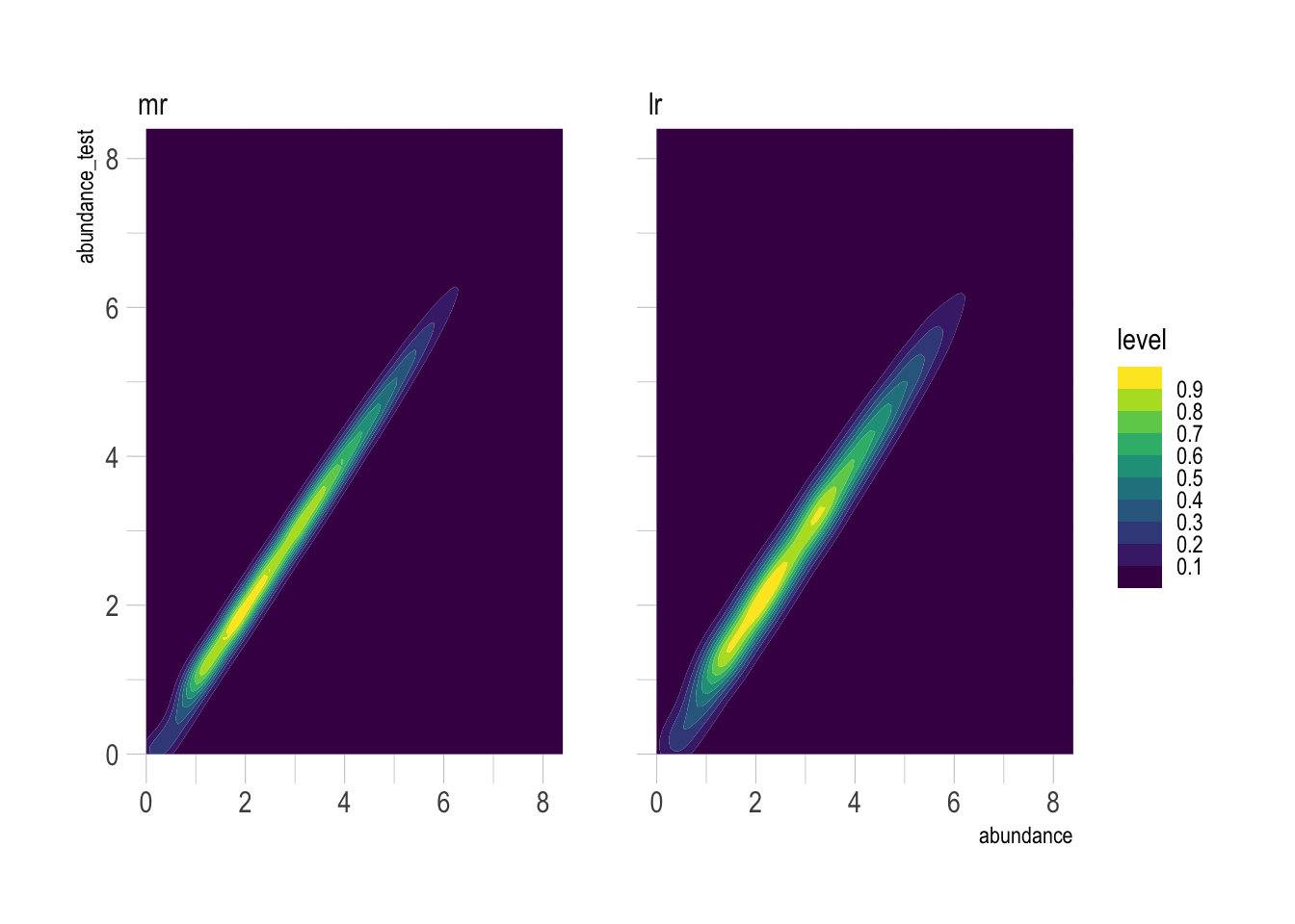
At lower resolutions, the difference is positively skewed, which means that abundance is higher than abundance_test.
species_table_unnested %>%
  drop_na(diff) %>%
  ggplot(aes(diff)) +
  geom_histogram() +
  facet_wrap(~resolution, scale = "free_y", ncol = 1)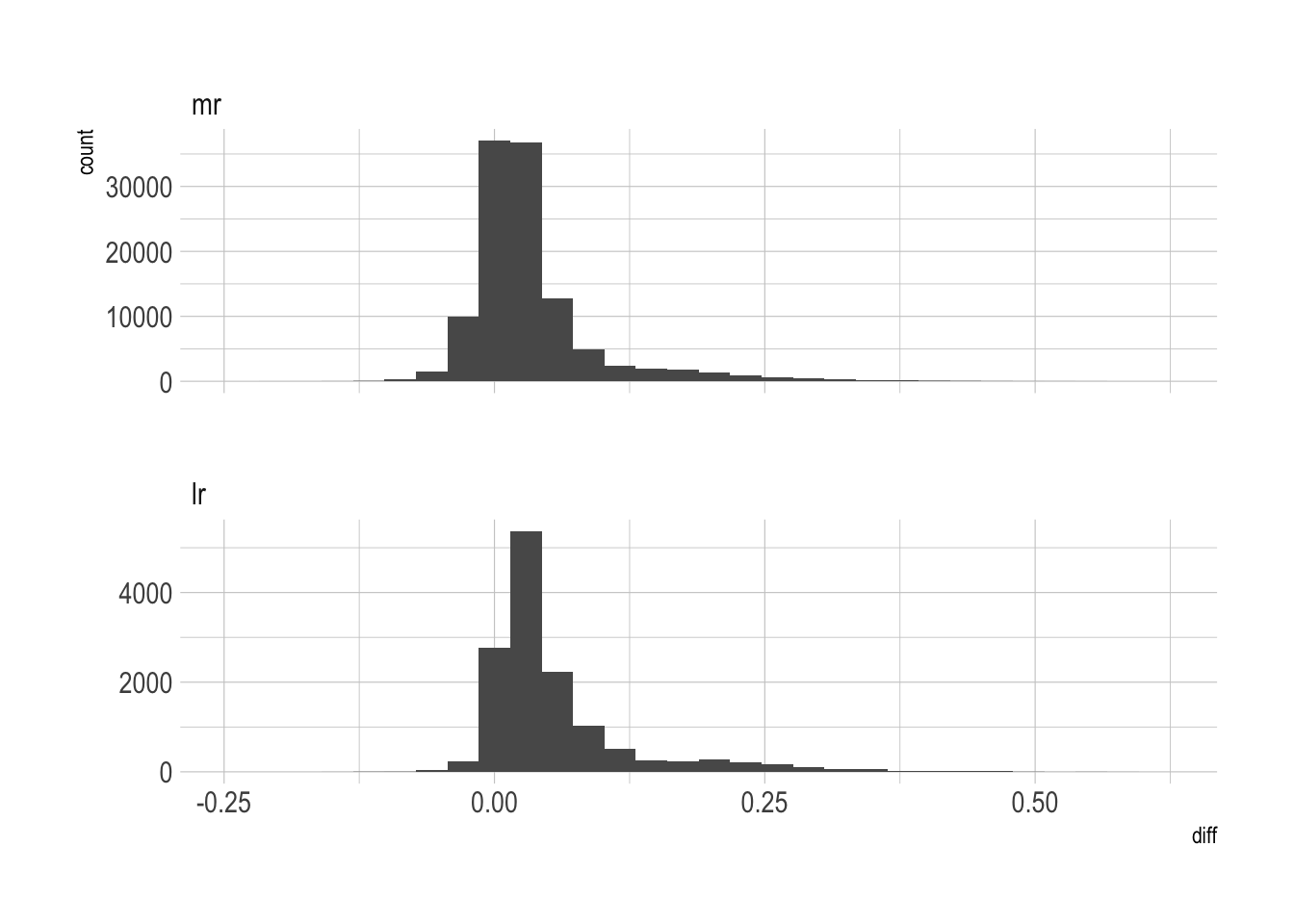
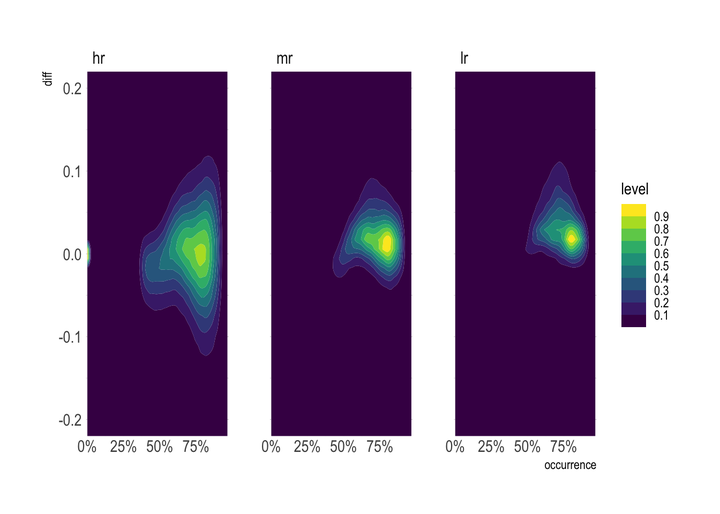
At the highest resolution, diff is heteroskedastic. At lower resolutions, there are patterns to the error. When occurrence is between 50% and 90%, diff is again skewed positively.
species_table_unnested %>%
  drop_na(occurrence, diff) %>%
  ggplot(aes(occurrence, diff)) +
  geom_density_2d_filled(contour_var = "ndensity") +
  facet_wrap(~resolution) +
  coord_cartesian(ylim = c(-.2, .2)) +
  scale_x_percent() +
  guides(fill = guide_colorsteps())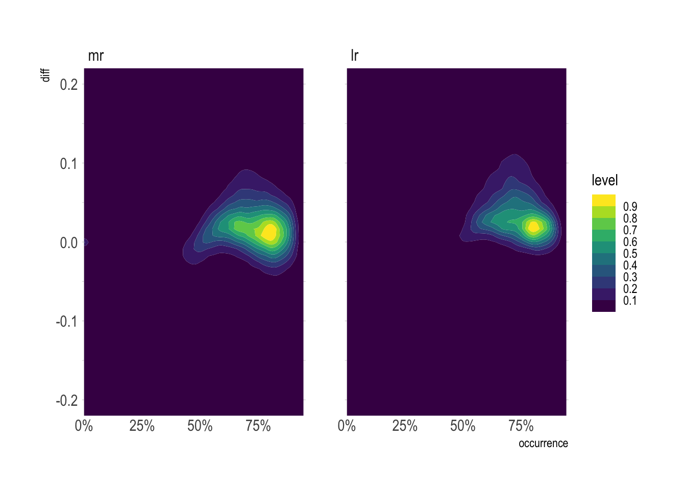
This was a useful exercise for me to understand how the geographic resolution and other aggregation of the data can affect estimated metrics, specifically in the citizen science context.
Update
I made an issue on the ebirdst Github page and talked to one of the maintainers about their definitions of count and abundance. I now have a much stronger understanding of these variables.
The following code reproduces the graph I attached to the issue:
library(hrbrthemes)
theme_set(theme_ipsum())

norcar_table <- crossing(species = c("Northern Cardinal"),
                          metric = c("occurrence", "count", "abundance"),
                          resolution = c("hr"))

norcar_metrics <- norcar_table %>%
  mutate(data = pmap(list(species, metric, resolution), ~get_species_metric(..1, ..2, ..3))) %>%
  mutate(resolution = fct_relevel(resolution, c("hr", "mr", "lr"))) %>%
  arrange(species, metric, resolution)
## 0.497 sec elapsed
## 23.346 sec elapsed
## 2.818 sec elapsed
## 0.578 sec elapsed
## 23.334 sec elapsed
## 2.875 sec elapsed
## 0.453 sec elapsed
## 24.111 sec elapsed
## 2.827 sec elapsednorcar_metrics_unnested <- norcar_metrics %>%
unnest(data)
norcar_metrics_wide <- norcar_metrics_unnested %>%
select(species, date, x, y, metric_desc, value) %>%
pivot_wider(id_cols = c(species, date, x, y, metric_desc),
names_from = metric_desc,
values_from = value)
plot_1 <- norcar_metrics_wide %>%
drop_na(occurrence, count) %>%
ggplot(aes(occurrence, count)) +
geom_density_2d_filled(contour_var = "ndensity") +
scale_x_percent() +
coord_cartesian(ylim = c(0, 12)) +
guides(fill = "none") +
theme_bw()
plot_2 <- norcar_metrics_wide %>%
drop_na() %>%
ggplot(aes(occurrence, abundance)) +
geom_density_2d_filled(contour_var = "ndensity") +
scale_x_percent() +
coord_cartesian(ylim = c(0, 12)) +
guides(fill = "none") +
theme_bw()
plot_3 <- norcar_metrics_wide %>%
drop_na() %>%
ggplot(aes(count, abundance)) +
geom_density_2d_filled(contour_var = "ndensity") +
geom_abline() +
coord_cartesian(xlim = c(0, 12),
ylim = c(0, 12)) +
guides(fill = "none") +
theme_bw()
layout <- "
AACC
BBCC
"
plot_1 + plot_2 + plot_3 +
plot_layout(guides = 'collect', design = layout) +
plot_annotation(title = "Northern Cardinal in Allegheny County Pennsylvania")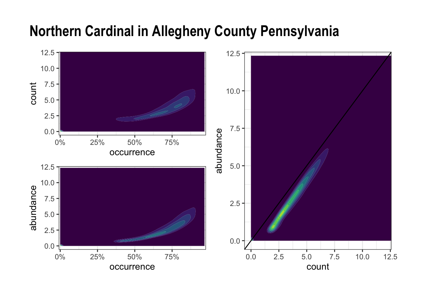
Citations
Fink, D., T. Auer, A. Johnston, M. Strimas-Mackey, O. Robinson, S. Ligocki, W. Hochachka, C. Wood, I. Davies, M. Iliff, L. Seitz. 2020. eBird Status and Trends, Data Version: 2019; Released: 2020 Cornell Lab of Ornithology, Ithaca, New York. https://doi.org/10.2173/ebirdst.2019