USL in the 538 Global Club Soccer Rankings
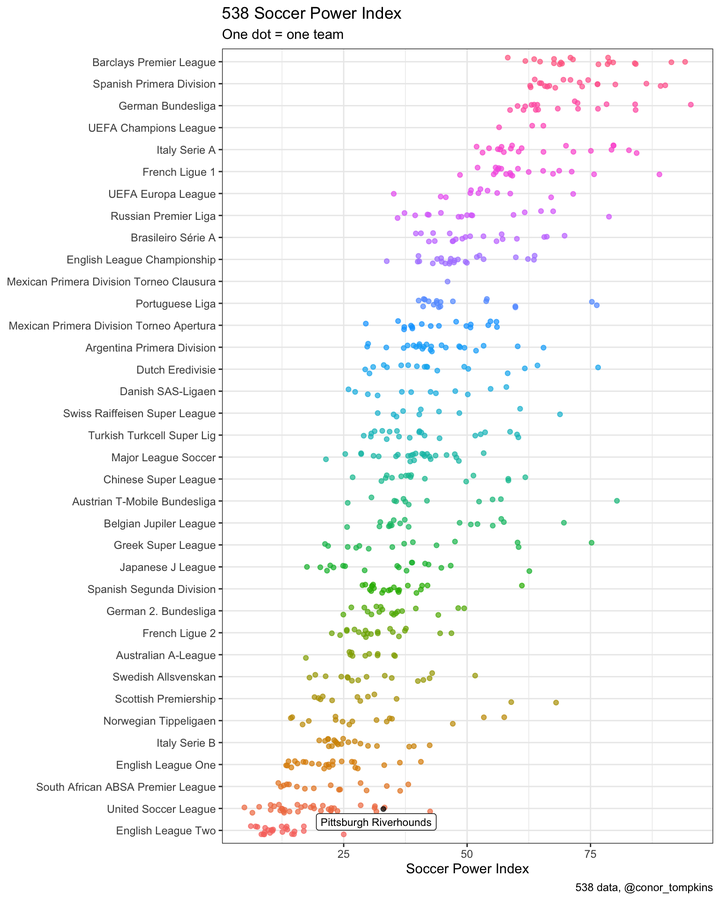
This post was originally run with data from August 2018. 538 does not provide historical rankings, so I had to rerun the code with September 2020 data when I migrated my blog.
538 recently added the United Soccer League to their Soccer Power Index ratings. I’m a Riverhounds fan, so I wanted to see how the team compared to teams from leagues around the world.
library(tidyverse)
library(ggrepel)

theme_set(theme_bw())
df <- read_csv("https://projects.fivethirtyeight.com/soccer-api/club/spi_global_rankings.csv", progress = FALSE) %>%
group_by(league) %>%
mutate(league_spi = median(spi)) %>%
ungroup() %>%
mutate(league = fct_reorder(league, league_spi))
df## # A tibble: 633 x 8
## rank prev_rank name league off def spi league_spi
## <dbl> <dbl> <chr> <fct> <dbl> <dbl> <dbl> <dbl>
## 1 1 1 Bayern Munich German Bundesliga 3.42 0.27 95.3 66.4
## 2 2 2 Manchester Ci… Barclays Premier… 3.09 0.24 94.2 71.2
## 3 3 3 Liverpool Barclays Premier… 2.84 0.33 91.4 71.2
## 4 4 4 Barcelona Spanish Primera … 2.88 0.43 90.1 70.2
## 5 5 5 Real Madrid Spanish Primera … 2.52 0.32 89.2 70.2
## 6 6 6 Paris Saint-G… French Ligue 1 2.89 0.51 89.0 58.8
## 7 7 8 Atletico Madr… Spanish Primera … 2.28 0.35 86.3 70.2
## 8 8 10 Internazionale Italy Serie A 2.51 0.570 84.3 60.8
## 9 9 9 Chelsea Barclays Premier… 2.44 0.54 84.2 71.2
## 10 10 12 RB Leipzig German Bundesliga 2.45 0.55 84.1 66.4
## # … with 623 more rowsdf %>%
ggplot(aes(spi, league)) +
geom_jitter(aes(color = league), show.legend = FALSE,
height = .2,
alpha = .7) +
geom_jitter(data = df %>% filter(name == "Pittsburgh Riverhounds"),
show.legend = FALSE,
height = .2,
alpha = .7) +
geom_label_repel(data = df %>% filter(name == "Pittsburgh Riverhounds"),
aes(label = name),
size = 3,
show.legend = FALSE,
force = 6) +
labs(title = "538 Soccer Power Index",
subtitle = "One dot = one team",
y = NULL,
x = "Soccer Power Index",
caption = "538 data, @conor_tompkins")
df %>%
  ggplot(aes(spi, league)) +
  geom_jitter(aes(color = league), show.legend = FALSE,
              height = .2,
              alpha = .7) +
  labs(title = "538 Soccer Power Index",
       subtitle = "One dot = one team",
       y = NULL,
       x = "Soccer Power Index",
       caption = "538 data, @conor_tompkins")
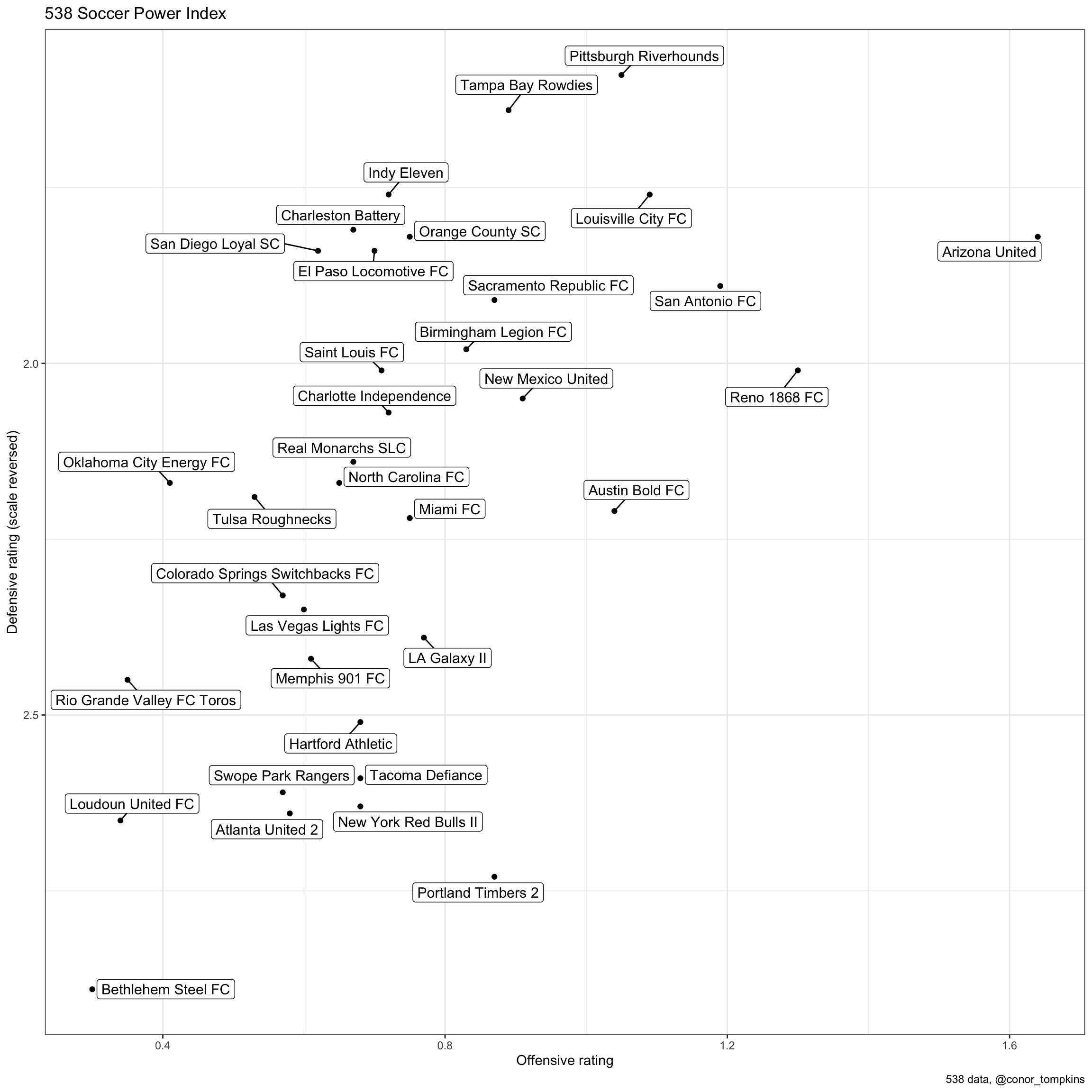
This shows the offensive and defensive ratings of each USL team. The Riverhounds are squarely in the #LilleyBall quadrant.
df %>%
  filter(league == "United Soccer League") %>%
  ggplot(aes(off, def, label = name)) +
  geom_point() +
  geom_label_repel(size = 4,
                   force = 4) +
  scale_y_reverse() +
  labs(title = "538 Soccer Power Index",
       y = "Defensive rating (scale reversed)",
       x = "Offensive rating",
       caption = "538 data, @conor_tompkins")