Pittsburgh Riverhounds under Coach Lilley
I have been a season-ticket holder with the Pittsburgh Riverhounds for a couple seasons now. The stadium has a great fan experience, and the team has gotten a lot better over the past few years. A major part of that is the head coach, Bob Lilley. I will use some data from American Soccer Analysis to show how the Riverhounds have improved. Their website has an explainer on expected goals and other metrics they calculate.
Load libraries and configure settings:
library(tidyverse)
library(janitor)
library(hrbrthemes)
library(ggrepel)

theme_set(theme_ipsum(base_size = 18))

#source https://app.americansocceranalysis.com/#!/
I pulled a CSV of team-level goal metrics for the last 4 USL seasons from the ASA website. This shows the available data:
usl <- read_csv("data/american_soccer_analysis_uslc_xgoals_teams_2021-03-17.csv") %>%
  clean_names() %>%
  select(-x1) %>%
  mutate(coach = case_when(team == "PIT" & season >= 2018 ~ "Lilley",
                           team == "PIT" & season < 2018 ~ "Brandt",
                           TRUE ~ NA_character_))

glimpse(usl)
## Rows: 134
## Columns: 15
## $ team <chr> "PHX", "CIN", "RNO", "LOU", "HFD", "PIT", "SLC", "SA", "TBR", …
## $ season <dbl> 2019, 2018, 2020, 2020, 2020, 2020, 2017, 2020, 2020, 2020, 20…
## $ games <dbl> 34, 34, 16, 16, 16, 16, 32, 16, 16, 16, 34, 15, 16, 34, 34, 34…
## $ sht_f <dbl> 16.79, 12.68, 16.06, 15.06, 10.31, 10.81, 11.88, 14.81, 12.63,…
## $ sht_a <dbl> 13.32, 15.15, 14.94, 9.56, 12.19, 7.81, 11.41, 12.44, 9.38, 13…
## $ gf <dbl> 2.53, 2.06, 2.69, 1.75, 1.88, 2.38, 1.84, 1.88, 1.56, 2.75, 1.…
## $ ga <dbl> 1.00, 0.97, 1.31, 0.75, 1.44, 0.63, 0.91, 0.75, 0.63, 1.19, 0.…
## $ gd <dbl> 1.53, 1.09, 1.38, 1.00, 0.44, 1.75, 0.94, 1.13, 0.94, 1.56, 0.…
## $ x_gf <dbl> 2.02, 1.45, 2.28, 1.43, 1.34, 1.63, 1.46, 1.55, 1.59, 2.36, 1.…
## $ x_ga <dbl> 1.41, 1.28, 1.52, 1.04, 1.33, 0.92, 1.33, 1.15, 0.84, 1.34, 0.…
## $ x_gd <dbl> 0.61, 0.17, 0.76, 0.39, 0.01, 0.71, 0.13, 0.40, 0.76, 1.02, 0.…
## $ gd_x_gd <dbl> 0.92, 0.92, 0.62, 0.61, 0.43, 1.04, 0.81, 0.72, 0.18, 0.55, 0.…
## $ pts <dbl> 2.29, 2.26, 2.25, 2.19, 2.19, 2.13, 2.09, 2.06, 2.06, 2.00, 2.…
## $ x_pts <dbl> 1.75, 1.47, 1.86, 1.62, 1.41, 1.85, 1.44, 1.64, 1.85, 1.95, 1.…
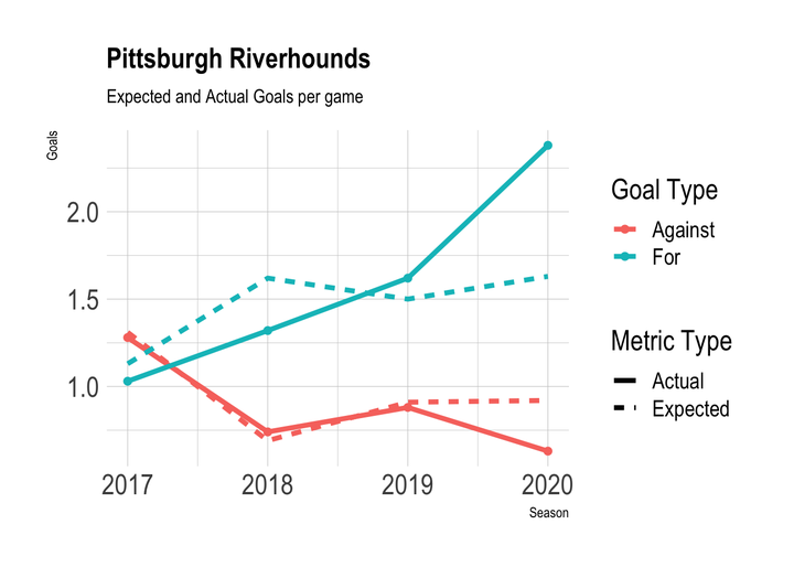
## $ coach <chr> NA, NA, NA, NA, NA, "Lilley", NA, NA, NA, NA, "Lilley", NA, NA…The Riverhound’s statistics show clear improvement in 2018 when Lilley took over from Brandt. The team immediately began scoring more than they allowed. The team’s expected goals for and against also improved, which shows that the improvement wasn’t a matter of luck.
goal_data <- usl %>%
  filter(team == "PIT") %>%
  select(team, season, gf, x_gf, ga, x_ga) %>%
  pivot_longer(cols = c(gf, x_gf, ga, x_ga), names_to = "g_type", values_to = "g_value") %>%
  mutate(goal_type = case_when(str_detect(g_type, "gf$") ~ "For",
                               TRUE ~ "Against")) %>%
  mutate(metric_type = case_when(str_detect(g_type, "^x_") ~ "Expected",
                                 TRUE ~ "Actual"))

goal_data %>%
  ggplot(aes(season, g_value, color = goal_type, lty = metric_type)) +
  geom_line(size = 1.5) +
  geom_point(data = filter(goal_data, metric_type == "Actual"), size = 2) +
  labs(title = "Pittsburgh Riverhounds",
       subtitle = "Expected and Actual Goals per game",
       x = "Season",
       y = "Goals",
       color = "Goal Type",
       lty = "Metric Type")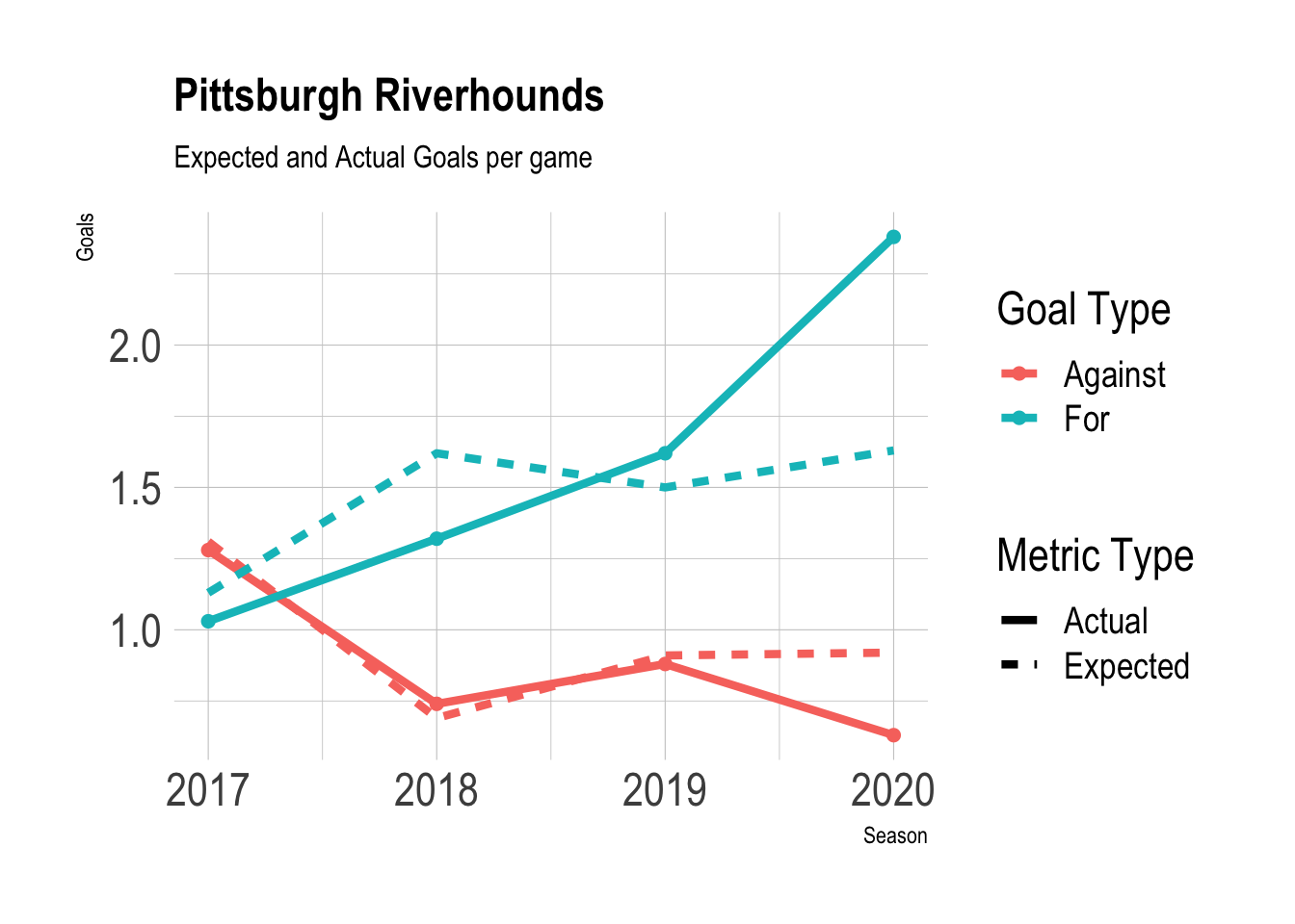
This shows that in terms of expected goal difference, the Riverhounds became one of the top teams in the USL once Lilley took over.
usl %>%
  ggplot(aes(season, x_gd, group = team)) +
  geom_hline(yintercept = 0, size = 1, lty = 2) +
  geom_line(color = "black", alpha = .2) +
  geom_line(data = filter(usl, team == "PIT"),
            color = "gold", size = 2) +
  geom_point(data = filter(usl, team == "PIT"),
             aes(fill = coach),
             shape = 21, size = 4) +
  scale_fill_manual(values = c("grey", "gold")) +
  #coord_fixed(ratio = .5) +
  labs(title = "xG difference per game",
       x = "Season",
       y = "xG Difference",
       fill = "Riverhounds Coach",
       caption = "Grey lines show other USL teams")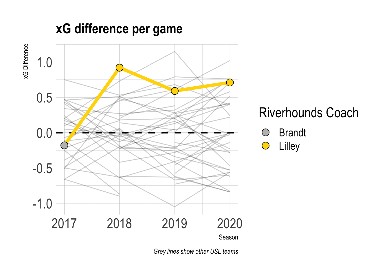
Lilley’s Riverhounds are consistently better than league average in terms of expected goals.
usl %>%
  ggplot(aes(x_gd)) +
  #geom_histogram(binwidth = .2) +
  geom_vline(data = filter(usl, team == "PIT"), aes(xintercept = x_gd), size = 3) +
  geom_vline(data = filter(usl, team == "PIT"), aes(xintercept = x_gd, color = coach),
             size = 2.5, key_glyph = "rect") +
  geom_density(aes(y = ..count.. * .2), fill = "white", alpha = 1) +
  geom_vline(xintercept = 0, lty = 2) +
  geom_hline(yintercept = 0) +
  scale_color_manual(values = c("grey", "gold")) +
  scale_x_continuous(expand = c(0,0)) +
  scale_y_continuous(expand = c(0,0)) +
  coord_cartesian(ylim = c(0, 25)) +
  #coord_fixed(ratio = .1) +
  labs(title = "xG Difference Per Game",
       subtitle = "Distribution of all USL teams 2017-2020",
       x = "xG",
       y = "Number of teams",
       color = "Riverhounds Coach") +
  theme(legend.key = element_rect(color = "black"))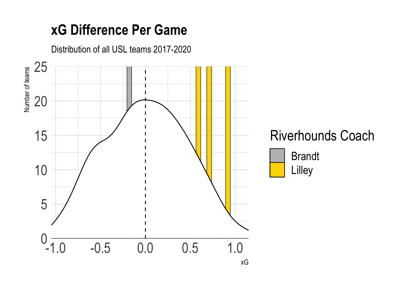
While the 2020 Riverhounds were a very good team, they were not quite as good as their plain goals for/against would show. This graph shows that they were fortunate to do as well as they did (which, again, was very well).
usl %>%
  mutate(logo = case_when(team == "PIT" ~ "data/pit_logo.png",
                          TRUE ~ NA_character_)) %>%
  ggplot(aes(x_gd, gd)) +
  geom_abline(lty = 2) +
  geom_point(alpha = .3) +
  ggimage::geom_image(aes(image = logo)) +
  geom_label_repel(data = filter(usl, team == "PIT"),
                   aes(label = season, fill = coach),
                   force = 5,
                   key_glyph = "rect") +
  annotate("text", label = "Under-performing",
           x = .75, y = -1.5) +
  annotate("text", label = "Over-performing",
           x = -1, y = 1.5) +
  tune::coord_obs_pred() +
  scale_fill_manual(values = c("grey", "gold")) +
  labs(title = "Goal and xG difference per game",
       x = "xG Difference",
       y = "Goal Difference",
       fill = "Riverhounds Coach") +
  theme(legend.key = element_rect(color = "black"))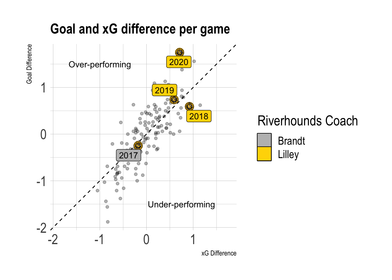
This shows that the 2020 Riverhounds were probably one of the most fortunate teams in the league, in addition to being very good.
usl %>%
  ggplot(aes(season, gd_x_gd, group = team)) +
  geom_hline(yintercept = 0, lty = 2) +
  geom_line(color = "black", alpha = .2) +
  geom_line(data = filter(usl, team == "PIT"),
            color = "gold", size = 2) +
  geom_point(data = filter(usl, team == "PIT"),
             aes(fill = coach, group = team),
             shape = 21, size = 4, color = "black") +
  scale_fill_manual(values = c("grey", "gold")) +
  coord_cartesian(ylim = c(-1.5, 1.5)) +
  #coord_fixed(ratio = .5) +
  labs(title = "Goal difference - xG difference",
       subtitle = "Per game",
       x = "Season",
       y = substitute(paste("" %<-% "", "Under-performing", "  |  ", "Over-performing", "" %->% "")),
       fill = "Riverhounds Coach",
       caption = "Grey lines show other USL teams")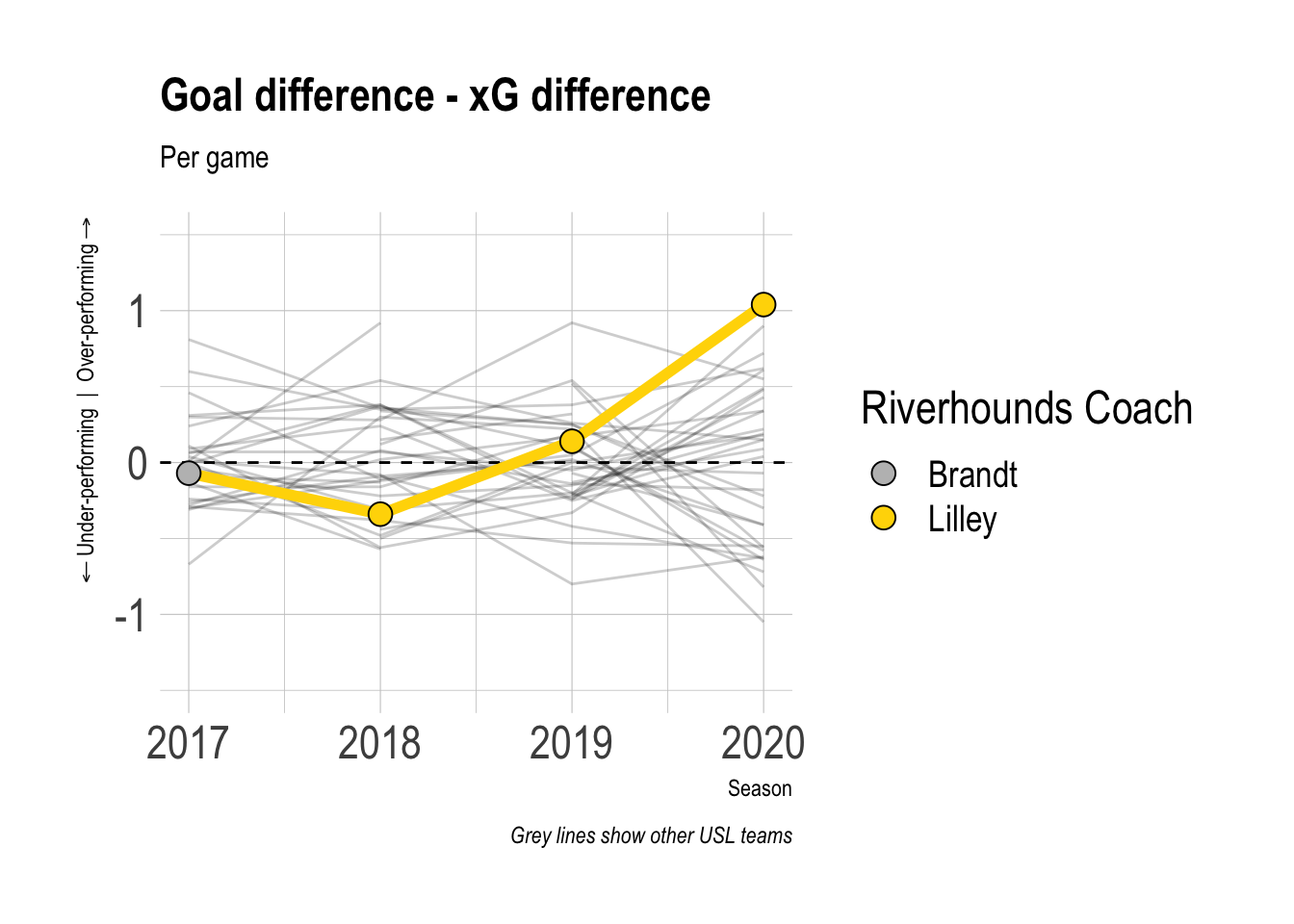
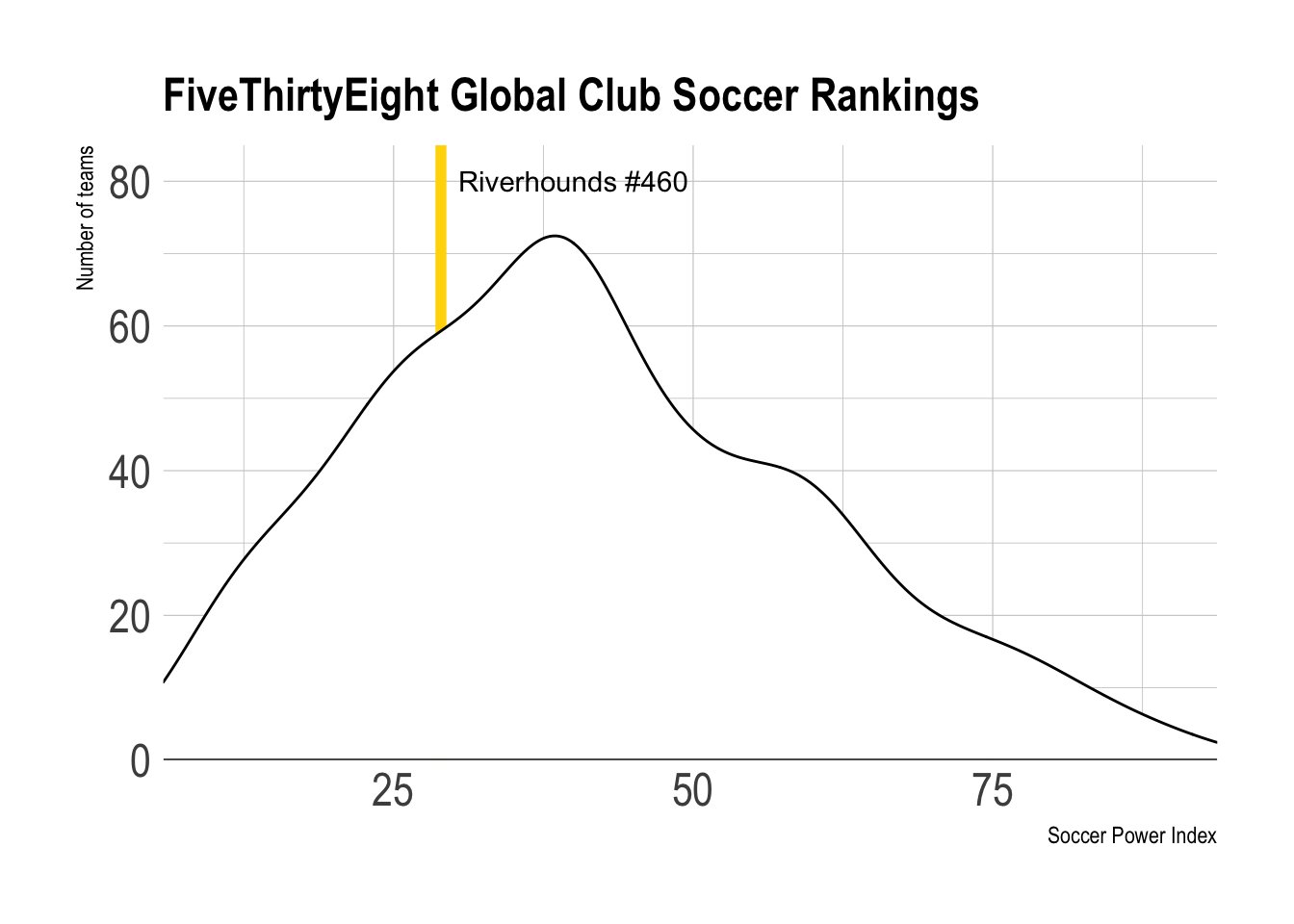
In FiveThirtyEights’ Global Soccer Power Index, the Riverhounds will begin the 2021 season ranked around #460 out of 639 teams.
fte_rankings <- read_csv("data/spi_global_rankings.csv")

fte_rankings %>%
  ggplot(aes(spi)) +
  geom_vline(data = filter(fte_rankings, name == "Pittsburgh Riverhounds"),
             aes(xintercept = spi), size = 2, color = "gold") +
  geom_density(aes(y = ..count.. * 5), fill = "white") +
  #geom_histogram(binwidth = 5) +
  geom_hline(yintercept = 0) +
  scale_x_continuous(expand = c(0,0)) +
  scale_y_continuous(expand = c(0,0)) +
  coord_cartesian(ylim = c(0, 85)) +
  annotate("text", x = 40, y = 80, label = "Riverhounds #460") +
  labs(title = "FiveThirtyEight Global Club Soccer Rankings",
       x = "Soccer Power Index",
       y = "Number of teams")