Modeling Pittsburgh House Sales Linear
In this post I will be modeling house (land parcel) sales in Pittsburgh. The data is from the WPRDC’s Parcels n’at dashboard.
The goal is to use linear modeling to predict the sale price of a house using features of the house and the property.
This code sets up the environment and loads the libraries I will use.
#load libraries
library(tidyverse)
library(scales)
library(caret)
library(broom)
library(modelr)
library(rsample)
library(janitor)
library(vroom)

#set up environment
options(scipen = 999, digits = 5)

theme_set(theme_bw())
This reads the data and engineers some features.
#read in data
df <- vroom("data/assessments.csv", col_types = cols(.default = "c")) %>%
  clean_names() %>%
  mutate(across(.cols = c(saleprice, finishedlivingarea, lotarea, yearblt,
                          bedrooms, fullbaths, halfbaths), parse_number))

#glimpse(df)

# df %>%
#   select(saleprice, finishedlivingarea, lotarea, yearblt, bedrooms, fullbaths, halfbaths) %>%
#   glimpse()
#
# df %>%
#   select(contains("muni"))
df <- df %>%
mutate(munidesc = str_replace(munidesc, " - PITTSBURGH", "")) %>%
mutate(finishedlivingarea_log10 = log10(finishedlivingarea),
lotarea_log10 = log10(lotarea),
saleprice_log10 = log10(saleprice)) %>%
select(parid, classdesc, munidesc, schooldesc, neighdesc, taxdesc,
usedesc, homesteadflag, farmsteadflag, styledesc,
yearblt, extfinish_desc, roofdesc, basementdesc,
gradedesc, conditiondesc, stories, totalrooms, bedrooms,
fullbaths, halfbaths, heatingcoolingdesc, fireplaces,
bsmtgarage, finishedlivingarea, finishedlivingarea_log10,
lotarea, lotarea_log10, saledate,
saleprice, saleprice_log10)
#create grade vectors
grades_standard <- c("average -", "average", "average +",
"good -", "good", "good +",
"very good -", "very good", "very good +")
grades_below_average_or_worse <- c("poor -", "poor", "poor +",
"below average -", "below average", "below average +")
grades_excellent_or_better <- c("excellent -", "excellent", "excellent +",
"highest cost -", "highest cost", "highest cost +")
#subset data and engineer features
df <- df %>%
filter(classdesc == "RESIDENTIAL",
saleprice > 100,
str_detect(munidesc, "Ward"),
finishedlivingarea > 0,
lotarea > 0) %>%
select(parid, munidesc, schooldesc, neighdesc, taxdesc,
usedesc, homesteadflag, farmsteadflag, styledesc,
yearblt, extfinish_desc, roofdesc, basementdesc,
heatingcoolingdesc, gradedesc, conditiondesc, stories,
totalrooms, bedrooms, fullbaths, halfbaths, fireplaces,
bsmtgarage, finishedlivingarea_log10, lotarea_log10,
saleprice_log10, saledate) %>%
mutate(usedesc = fct_lump(usedesc, n = 5),
styledesc = fct_lump(styledesc, n = 10),
#clean up and condense gradedesc
gradedesc = str_to_lower(gradedesc),
gradedesc = case_when(gradedesc %in% grades_below_average_or_worse ~ "below average + or worse",
gradedesc %in% grades_excellent_or_better ~ "excellent - or better",
gradedesc %in% grades_standard ~ gradedesc),
gradedesc = fct_relevel(gradedesc, c("below average + or worse", "average -", "average", "average +",
"good -", "good", "good +",
"very good -", "very good", "very good +", "excellent - or better")))
#replace missing character rows with "missing", change character columns to factor
df <- df %>%
mutate_if(is.character, replace_na, "missing") %>%
mutate_if(is.character, as.factor)
#select response and features
df <- df %>%
select(munidesc, usedesc, styledesc, conditiondesc, gradedesc,
finishedlivingarea_log10, lotarea_log10, yearblt, bedrooms,
fullbaths, halfbaths, saleprice_log10) %>%
na.omit()
#view data
glimpse(df)## Rows: 73,679
## Columns: 12
## $ munidesc <fct> 1st Ward , 1st Ward , 1st Ward , 1st Ward , …
## $ usedesc <fct> SINGLE FAMILY, SINGLE FAMILY, SINGLE FAMILY,…
## $ styledesc <fct> TOWNHOUSE, TOWNHOUSE, TOWNHOUSE, Other, Othe…
## $ conditiondesc <fct> EXCELLENT, EXCELLENT, EXCELLENT, AVERAGE, AV…
## $ gradedesc <fct> excellent - or better, excellent - or better…
## $ finishedlivingarea_log10 <dbl> 3.3034, 3.6170, 3.7042, 3.1173, 3.0993, 3.12…
## $ lotarea_log10 <dbl> 2.9978, 3.0461, 3.1477, 3.1173, 3.0993, 3.14…
## $ yearblt <dbl> 2015, 2012, 1920, 2015, 2007, 2007, 2015, 20…
## $ bedrooms <dbl> 3, 3, 2, 2, 2, 2, 2, 2, 2, 2, 2, 1, 1, 4, 6,…
## $ fullbaths <dbl> 3, 3, 3, 2, 2, 2, 2, 1, 2, 2, 2, 1, 1, 2, 2,…
## $ halfbaths <dbl> 1, 1, 1, 0, 0, 0, 0, 1, 0, 1, 1, 1, 1, 0, 0,…
## $ saleprice_log10 <dbl> 6.3010, 6.2544, 6.2380, 5.4695, 5.4033, 5.78…As shown in the data above, the model uses the following features to predict sale price:
- municipality name
- primary use of the parcel
- style of building
- condition of the structure
- grade of construction
- living area in square feet
- lot area in square feet
- year the house was built
- number of bedrooms
- number of full baths
- number of half-baths
This code sets up the data for cross validation.
#create initial split object
df_split <- initial_split(df, prop = .75)

#extract training dataframe
training_data_full <- training(df_split)

#extract testing dataframe
testing_data <- testing(df_split)

#find dimensions of training_data_full and testing_data
dim(training_data_full)
## [1] 55260 12dim(testing_data)## [1] 18419 12This code divides the data into training and testing sets.
set.seed(42)

#prep the df with the cross validation partitions
cv_split <- vfold_cv(training_data_full, v = 5)

cv_data <- cv_split %>%
  mutate(
    #extract train dataframe for each split
    train = map(splits, ~training(.x)),
    #extract validate dataframe for each split
    validate = map(splits, ~testing(.x))
  )

#view df
cv_data
## # 5-fold cross-validation
## # A tibble: 5 x 4
## splits id train validate
## <list> <chr> <list> <list>
## 1 <split [44.2K/11.1K]> Fold1 <tibble [44,208 × 12]> <tibble [11,052 × 12]>
## 2 <split [44.2K/11.1K]> Fold2 <tibble [44,208 × 12]> <tibble [11,052 × 12]>
## 3 <split [44.2K/11.1K]> Fold3 <tibble [44,208 × 12]> <tibble [11,052 × 12]>
## 4 <split [44.2K/11.1K]> Fold4 <tibble [44,208 × 12]> <tibble [11,052 × 12]>
## 5 <split [44.2K/11.1K]> Fold5 <tibble [44,208 × 12]> <tibble [11,052 × 12]>This builds the model to predict house sale price.
#build model using the train data for each fold of the cross validation
cv_models_lm <- cv_data %>%
  mutate(model = map(train, ~lm(formula = saleprice_log10 ~ ., data = .x)))

cv_models_lm
## # 5-fold cross-validation
## # A tibble: 5 x 5
## splits id train validate model
## <list> <chr> <list> <list> <lis>
## 1 <split [44.2K/11.1K]> Fold1 <tibble [44,208 × 12]> <tibble [11,052 × 12… <lm>
## 2 <split [44.2K/11.1K]> Fold2 <tibble [44,208 × 12]> <tibble [11,052 × 12… <lm>
## 3 <split [44.2K/11.1K]> Fold3 <tibble [44,208 × 12]> <tibble [11,052 × 12… <lm>
## 4 <split [44.2K/11.1K]> Fold4 <tibble [44,208 × 12]> <tibble [11,052 × 12… <lm>
## 5 <split [44.2K/11.1K]> Fold5 <tibble [44,208 × 12]> <tibble [11,052 × 12… <lm>#problem with factors split across training/validation
#https://stats.stackexchange.com/questions/235764/new-factors-levels-not-present-in-training-dataThis is where I begin to calculate metrics to judge how well my model is doing.
cv_prep_lm <- cv_models_lm %>%
  mutate(
    #extract actual sale price for the records in the validate dataframes
    validate_actual = map(validate, ~.x$saleprice_log10),
    #predict response variable for each validate set using its corresponding model
    validate_predicted = map2(.x = model, .y = validate, ~predict(.x, .y))
  )

#View data
cv_prep_lm
## # 5-fold cross-validation
## # A tibble: 5 x 7
## splits id train validate model validate_actual validate_predic…
## <list> <chr> <list> <list> <lis> <list> <list>
## 1 <split [4… Fold1 <tibble [… <tibble [1… <lm> <dbl [11,052]> <dbl [11,052]>
## 2 <split [4… Fold2 <tibble [… <tibble [1… <lm> <dbl [11,052]> <dbl [11,052]>
## 3 <split [4… Fold3 <tibble [… <tibble [1… <lm> <dbl [11,052]> <dbl [11,052]>
## 4 <split [4… Fold4 <tibble [… <tibble [1… <lm> <dbl [11,052]> <dbl [11,052]>
## 5 <split [4… Fold5 <tibble [… <tibble [1… <lm> <dbl [11,052]> <dbl [11,052]>#calculate fit metrics for each validate fold
cv_eval_lm <- cv_prep_lm %>%
mutate(validate_rmse = map2_dbl(model, validate, modelr::rmse),
validate_mae = map2_dbl(model, validate, modelr::mae))
cv_eval_lm <- cv_eval_lm %>%
mutate(fit = map(model, ~glance(.x))) %>%
unnest(fit)#view data
cv_eval_lm %>%
select(id, validate_mae, validate_rmse, adj.r.squared)## # A tibble: 5 x 4
## id validate_mae validate_rmse adj.r.squared
## <chr> <dbl> <dbl> <dbl>
## 1 Fold1 0.304 0.417 0.474
## 2 Fold2 0.305 0.417 0.474
## 3 Fold3 0.297 0.411 0.471
## 4 Fold4 0.304 0.418 0.474
## 5 Fold5 0.301 0.419 0.477Finally, this calculates how well the model did on the validation set.
#summarize fit metrics on cross-validated dfs
cv_eval_lm %>%
  select(validate_mae, validate_rmse, adj.r.squared) %>%
  summarize_all(mean)
## # A tibble: 1 x 3
## validate_mae validate_rmse adj.r.squared
## <dbl> <dbl> <dbl>
## 1 0.302 0.417 0.474#fit model on full training set
train_df <- cv_data %>%
select(train) %>%
unnest(train)
model_train <- lm(formula = saleprice_log10 ~ ., data = train_df)
model_train %>%
glance()## # A tibble: 1 x 12
## r.squared adj.r.squared sigma statistic p.value df logLik AIC BIC
## <dbl> <dbl> <dbl> <dbl> <dbl> <dbl> <dbl> <dbl> <dbl>
## 1 0.474 0.474 0.416 2293. 0 87 -1.20e5 2.39e5 2.40e5
## # … with 3 more variables: deviance <dbl>, df.residual <int>, nobs <int>This is the RMSE on the training set
#calculate rmse on training set
rmse(model_train, train_df)
## [1] 0.41561This shows the impact each term of the model has on the response variable. This is for the training data.
#visualize estimates for terms
model_train %>%
  tidy() %>%
  filter(term != "(Intercept)") %>%
  mutate(term = fct_reorder(term, estimate)) %>%
  ggplot(aes(term, estimate)) +
  geom_hline(yintercept = 0, linetype = 2, color = "red") +
  geom_point() +
  coord_flip()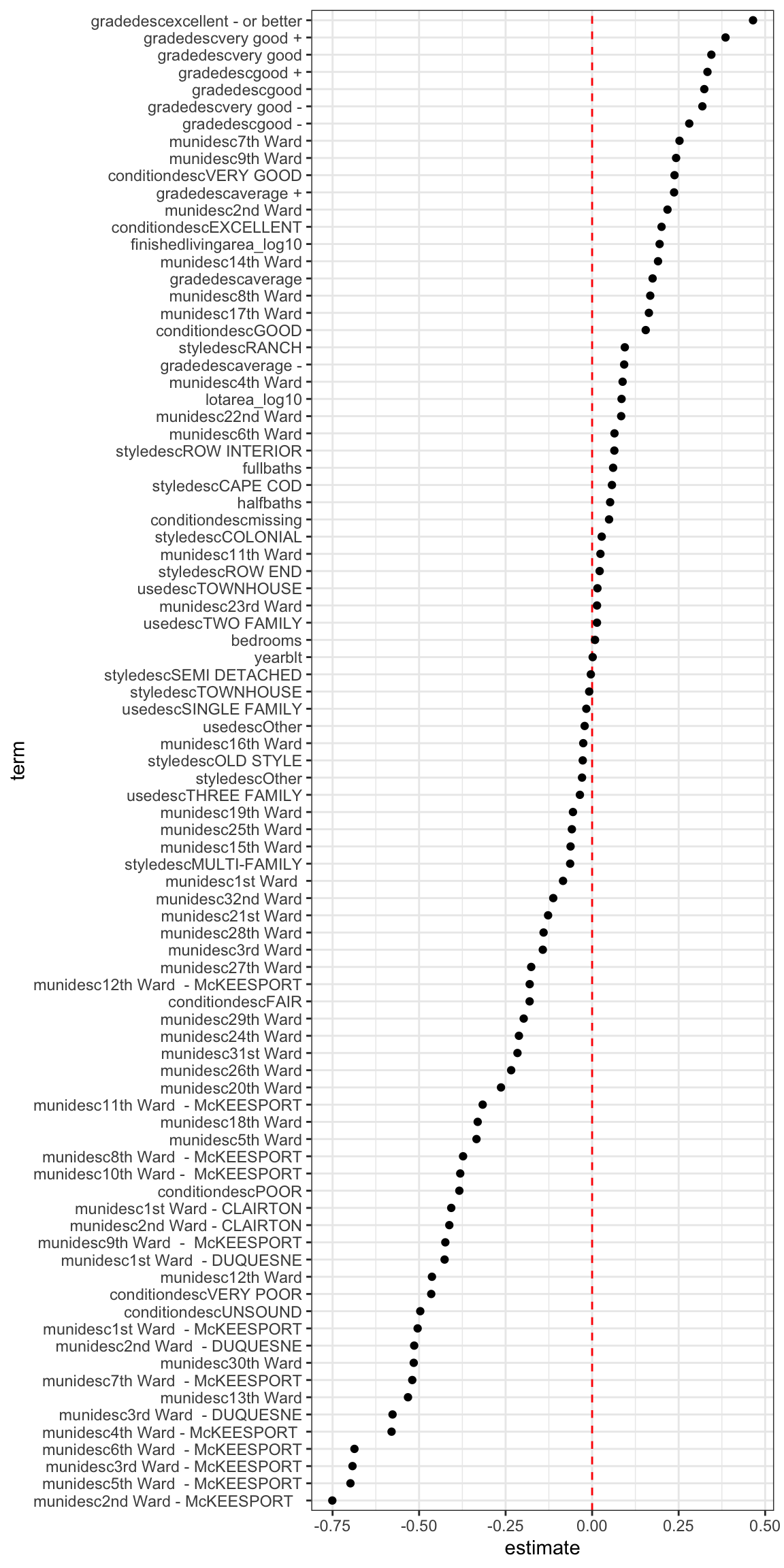
Next, I apply the model to the testing data to see how the model does out-of-sample.
#create dfs for train_data_small and validate_data
#train_data_small <- cv_prep_lm %>%
#  unnest(train) %>%
#  select(-id)

validate_df <- cv_prep_lm %>%
  select(validate) %>%
  unnest()
This creates the augmented dataframe and plots the actual price vs. the fitted price.
#visualize model on validate data
augment_validate <- augment(model_train, newdata = validate_df) %>%
  mutate(.resid = saleprice_log10 - .fitted)

#actual vs. fitted
cv_prep_lm %>%
  unnest(validate_actual, validate_predicted) %>%
  ggplot(aes(validate_actual, validate_predicted)) +
  geom_abline() +
  stat_density_2d(aes(fill = stat(level)), geom = "polygon") +
  geom_smooth(method = "lm") +
  scale_x_continuous(limits = c(2, 7)) +
  scale_y_continuous(limits = c(2, 7)) +
  coord_equal() +
  scale_fill_viridis_c()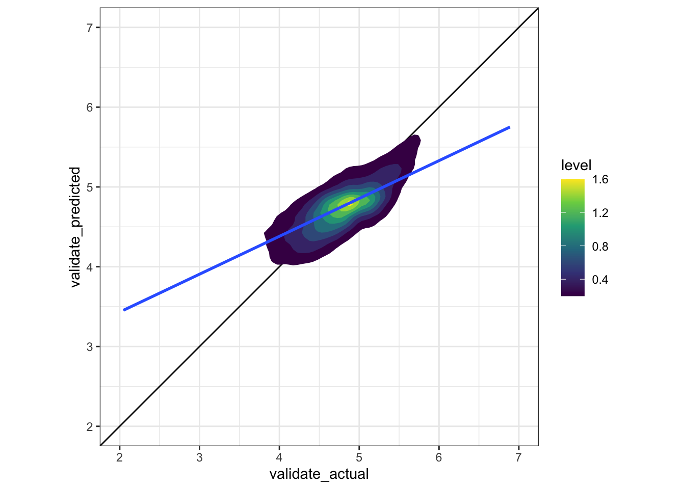
This distribution shows that the model overestimates the prices on many houses.
#distribution of residuals
augment_validate %>%
  ggplot(aes(.resid)) +
  geom_density() +
  geom_vline(xintercept = 0, color = "red", linetype = 2)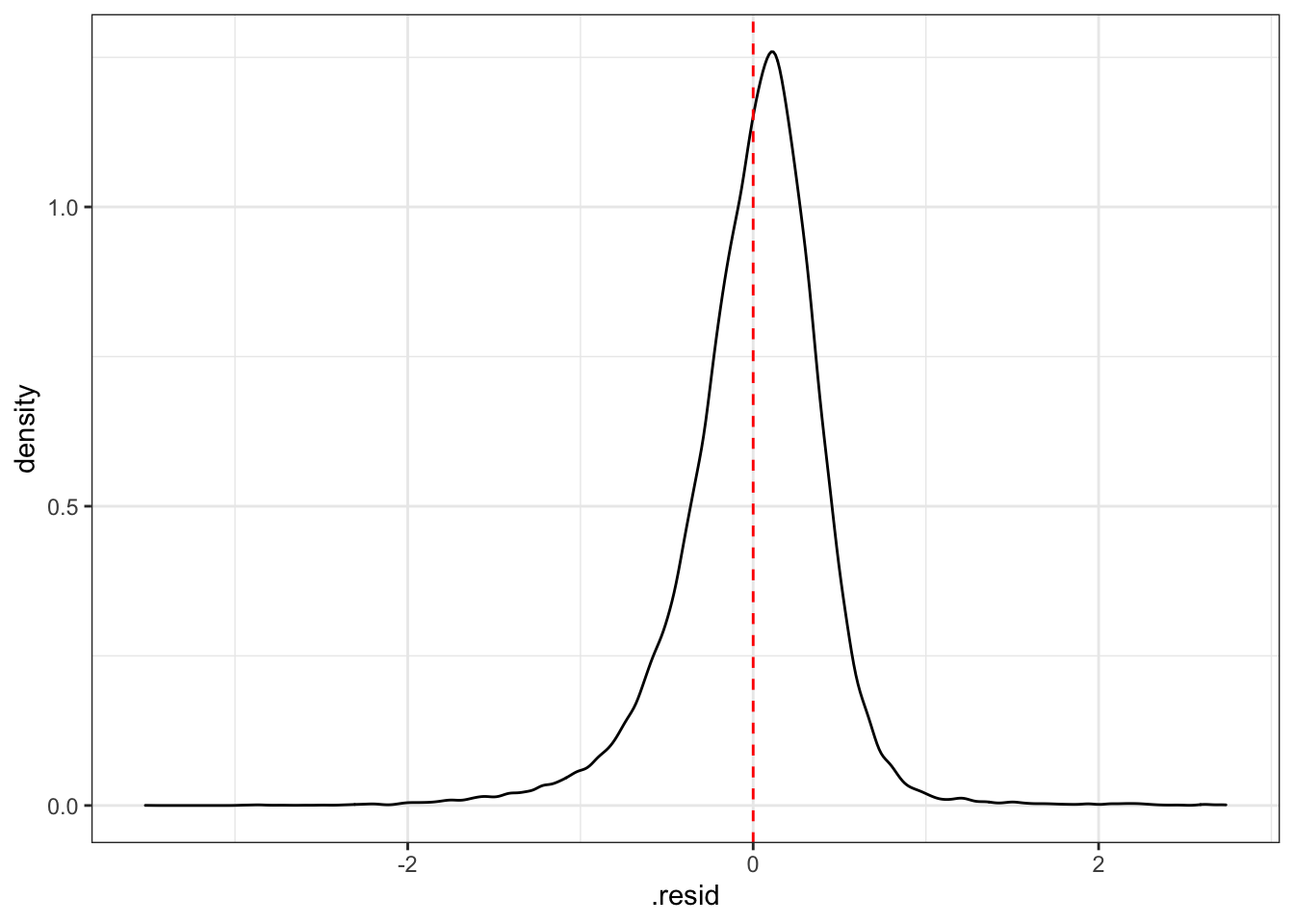
This shows that the residuals are correlated with the actual price, which indicates that the model is failing to account for some dynamic in the sale process.
#sale price vs. residuals
augment_validate %>%
  ggplot(aes(.resid, saleprice_log10)) +
  stat_density_2d(aes(fill = stat(level)), geom = "polygon") +
  geom_vline(xintercept = 0, color = "red", linetype = 2) +
  scale_fill_viridis_c()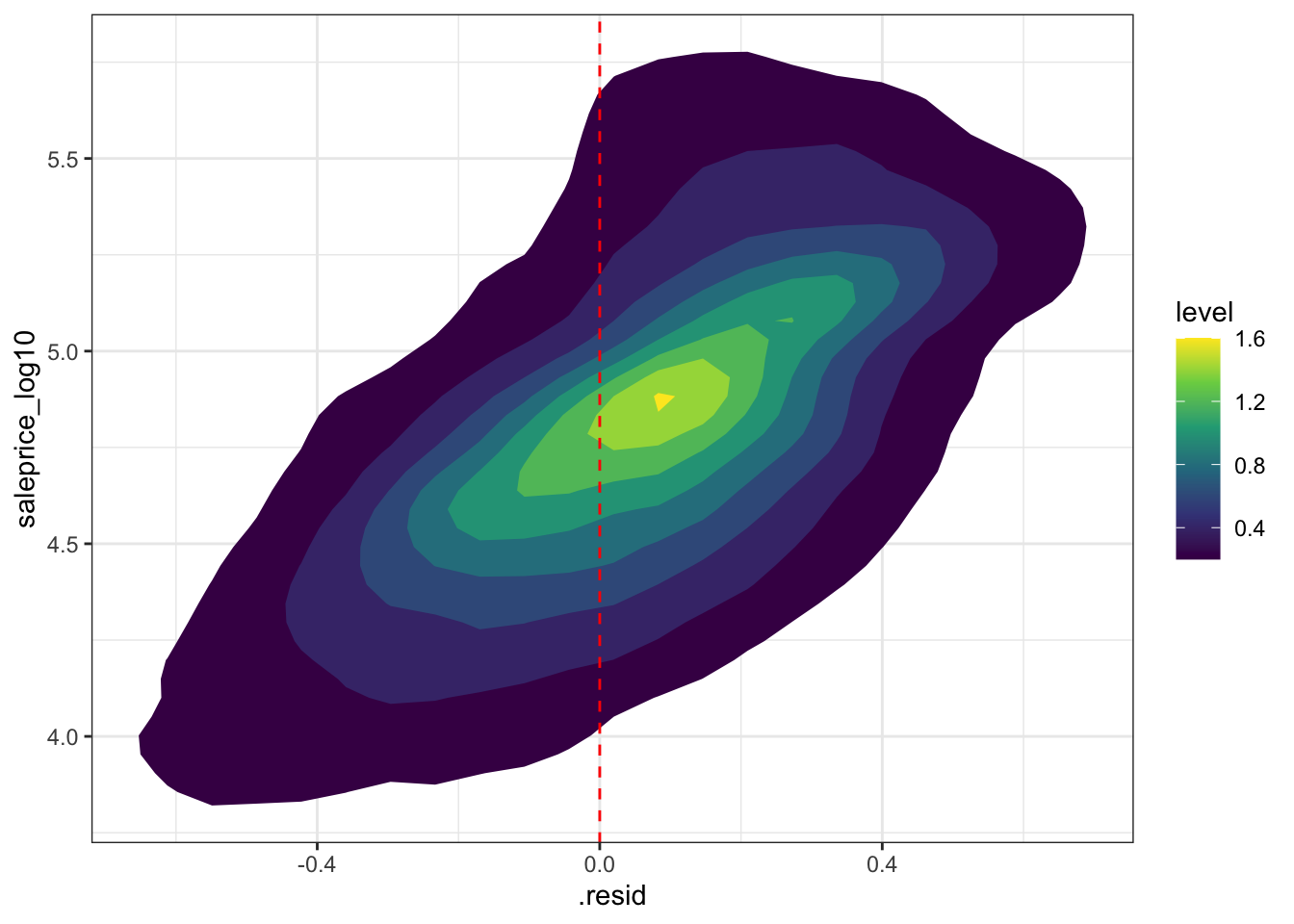
This calculates how well the model predicted sale price on out-of-sample testing data.
#calculate fit of model on test data
rmse(model_train, validate_df)
## [1] 0.41561mae(model_train, validate_df)## [1] 0.30157rsquare(model_train, validate_df)## [1] 0.47443