Exploring Allegheny County With Census Data

This post explores Allegheny County and Pennsylvania through census data. I use the tidycensus and sf packages to collect data from the census API and draw maps with the data.
Setup
library(tidyverse)
library(tidycensus)
library(tigris)
library(sf)
library(broom)
library(ggfortify)
library(viridis)
library(scales)
library(janitor)

options(tigris_use_cache = TRUE)

theme_set(theme_bw())

census_vars <- load_variables(2010, "sf1", cache = TRUE)
Collect data
tidycensus provides a wrapper for the U.S. Census API. You can request a wide variety of data, from economic measures to information about demography. The API also includes data about geographic regions.
This code creates a dataframe of some of the variables available through the census API.
vars <- load_variables(2016, "acs5", cache = TRUE)

vars
## # A tibble: 22,815 x 3
## name label concept
## <chr> <chr> <chr>
## 1 B00001_001 Estimate!!Total UNWEIGHTED SAMPLE COUNT OF THE PO…
## 2 B00002_001 Estimate!!Total UNWEIGHTED SAMPLE HOUSING UNITS
## 3 B01001_001 Estimate!!Total SEX BY AGE
## 4 B01001_002 Estimate!!Total!!Male SEX BY AGE
## 5 B01001_003 Estimate!!Total!!Male!!Under 5… SEX BY AGE
## 6 B01001_004 Estimate!!Total!!Male!!5 to 9 … SEX BY AGE
## 7 B01001_005 Estimate!!Total!!Male!!10 to 1… SEX BY AGE
## 8 B01001_006 Estimate!!Total!!Male!!15 to 1… SEX BY AGE
## 9 B01001_007 Estimate!!Total!!Male!!18 and … SEX BY AGE
## 10 B01001_008 Estimate!!Total!!Male!!20 years SEX BY AGE
## # … with 22,805 more rowsThis code requests information about the median income of census tracts in Allegheny County. The “geography” argument sets the level of geographic granularity.
allegheny <- get_acs(state = "PA",
                     county = "Allegheny County",
                     geography = "tract",
                     variables = c(median_income = "B19013_001"),
                     geometry = TRUE,
                     cb = FALSE)

head(allegheny)
## Simple feature collection with 6 features and 5 fields
## geometry type: MULTIPOLYGON
## dimension: XY
## bbox: xmin: -80.16148 ymin: 40.41478 xmax: -79.88377 ymax: 40.57546
## geographic CRS: NAD83
## GEOID NAME variable
## 1 42003563200 Census Tract 5632, Allegheny County, Pennsylvania median_income
## 2 42003980000 Census Tract 9800, Allegheny County, Pennsylvania median_income
## 3 42003564100 Census Tract 5641, Allegheny County, Pennsylvania median_income
## 4 42003461000 Census Tract 4610, Allegheny County, Pennsylvania median_income
## 5 42003437000 Census Tract 4370, Allegheny County, Pennsylvania median_income
## 6 42003981800 Census Tract 9818, Allegheny County, Pennsylvania median_income
## estimate moe geometry
## 1 29750 8141 MULTIPOLYGON (((-80.00469 4...
## 2 NA NA MULTIPOLYGON (((-79.90168 4...
## 3 145179 11268 MULTIPOLYGON (((-80.09943 4...
## 4 39063 6923 MULTIPOLYGON (((-80.16148 4...
## 5 106250 11871 MULTIPOLYGON (((-80.12246 4...
## 6 NA NA MULTIPOLYGON (((-79.90822 4...This code maps the data onto the census tracts. The st_erase function makes the rivers show up on the map (not working).
# st_erase <- function(x, y) {
#   st_difference(x, st_union(st_combine(y)))
# }

#allegheny_water <- area_water("PA", "Allegheny", class = "sf")

#allegheny_erase <- st_erase(allegheny, allegheny_water)

allegheny %>%
  ggplot(aes(fill = estimate, color = estimate)) +
  geom_sf() +
  scale_fill_viridis("Median household income", option = "magma", labels = comma) +
  scale_color_viridis("Median household income", option = "magma", labels = comma) +
  labs(title = "Allegheny County",
       subtitle = "American Community Survey") +
  theme(axis.text = element_blank())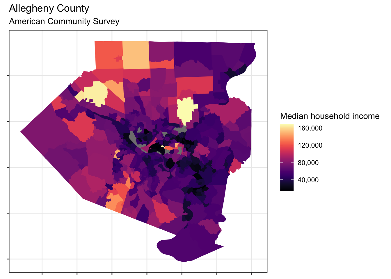
This code requests information about the ethnicities within each census tract. Then, it calculates the percentage of the entire population of a tract that each ethnicity makes up.
racevars <- c(White = "P005003",
              Black = "P005004",
              Asian = "P005006",
              Hispanic = "P004003")

get_decennial(geography = "tract",
                                variables = racevars,
                                state = "PA",
                                county = "Allegheny",
                                geometry = TRUE,
                                summary_var = "P001001") %>%
    mutate(value = value / summary_value,
           variable = str_c("percent_", tolower(variable))) -> allegheny_race

head(allegheny_race)
## Simple feature collection with 6 features and 5 fields
## geometry type: MULTIPOLYGON
## dimension: XY
## bbox: xmin: -80.12431 ymin: 40.54225 xmax: -79.99058 ymax: 40.61431
## geographic CRS: NAD83
## # A tibble: 6 x 6
## GEOID NAME variable value summary_value geometry
## <chr> <chr> <chr> <dbl> <dbl> <MULTIPOLYGON [°]>
## 1 42003… Census Tr… percent… 0.916 4865 (((-80.07936 40.58043, -80.0…
## 2 42003… Census Tr… percent… 0.00843 4865 (((-80.07936 40.58043, -80.0…
## 3 42003… Census Tr… percent… 0.0580 4865 (((-80.07936 40.58043, -80.0…
## 4 42003… Census Tr… percent… 0.0103 4865 (((-80.07936 40.58043, -80.0…
## 5 42003… Census Tr… percent… 0.878 6609 (((-80.06788 40.60846, -80.0…
## 6 42003… Census Tr… percent… 0.0172 6609 (((-80.06788 40.60846, -80.0…This code maps that data. The facet_wrap function creates a map for each ethnicity.
#allegheny_race <- st_erase(allegheny_race, allegheny_water)

allegheny_race %>%
  ggplot(aes(fill = value, color = value)) +
  facet_wrap(~variable) +
  geom_sf() +
  scale_fill_viridis("Percent", option = "magma", labels = percent) +
  scale_color_viridis("Percent", option = "magma", labels = percent) +
  theme(axis.text = element_blank())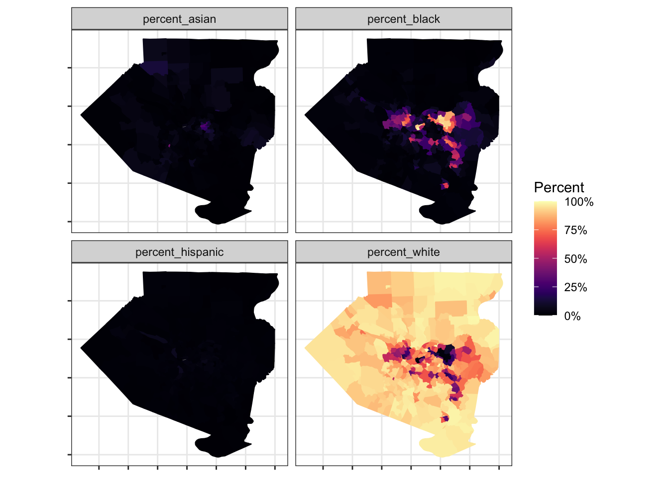
You can also request data for an entire state. This code requests the median income for each census tract in Pennsylvania.
pa <- get_acs(state = "PA",
                     geography = "tract",
                     variables = c(median_income = "B19013_001"),
                     geometry = TRUE)

head(pa)
## Simple feature collection with 6 features and 5 fields
## geometry type: MULTIPOLYGON
## dimension: XY
## bbox: xmin: -80.14905 ymin: 40.32178 xmax: -75.6175 ymax: 41.07083
## geographic CRS: NAD83
## GEOID NAME variable
## 1 42019910500 Census Tract 9105, Butler County, Pennsylvania median_income
## 2 42019912200 Census Tract 9122, Butler County, Pennsylvania median_income
## 3 42021000100 Census Tract 1, Cambria County, Pennsylvania median_income
## 4 42021012600 Census Tract 126, Cambria County, Pennsylvania median_income
## 5 42025020700 Census Tract 207, Carbon County, Pennsylvania median_income
## 6 42027010800 Census Tract 108, Centre County, Pennsylvania median_income
## estimate moe geometry
## 1 NA NA MULTIPOLYGON (((-80.04897 4...
## 2 93446 11356 MULTIPOLYGON (((-80.14905 4...
## 3 12907 1274 MULTIPOLYGON (((-78.92583 4...
## 4 47143 9880 MULTIPOLYGON (((-78.73584 4...
## 5 57939 4427 MULTIPOLYGON (((-75.71378 4...
## 6 53569 4123 MULTIPOLYGON (((-77.55509 4...pa %>%
ggplot(aes(fill = estimate, color = estimate)) +
geom_sf() +
scale_fill_viridis("Estimated median income", option = "magma", label = comma) +
scale_color_viridis("Estimated median income", option = "magma", label = comma) +
theme(axis.text = element_blank())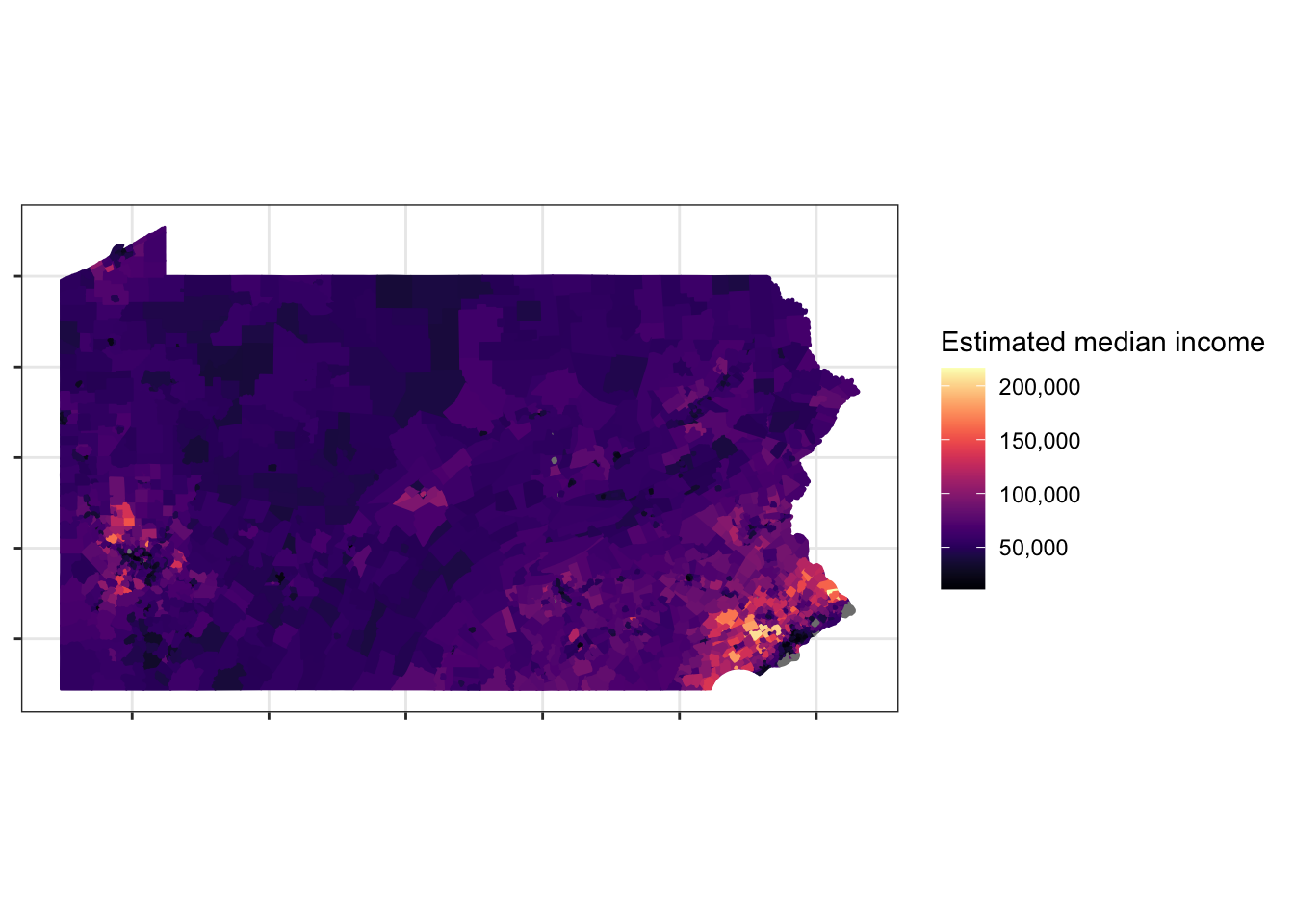
This code requests ethnicity data for each tract in Pennsylvania.
racevars <- c(White = "P005003",
              Black = "P005004",
              Asian = "P005006",
              Hispanic = "P004003")

get_decennial(geography = "tract",
                                variables = racevars,
                                state = "PA",
                                geometry = TRUE,
                                summary_var = "P001001") %>%
  mutate(value = value / summary_value,
         variable = str_c("percent_", tolower(variable))) -> pa_race

head(pa_race)
## Simple feature collection with 6 features and 5 fields
## geometry type: MULTIPOLYGON
## dimension: XY
## bbox: xmin: -80.12431 ymin: 40.54225 xmax: -79.99058 ymax: 40.61431
## geographic CRS: NAD83
## # A tibble: 6 x 6
## GEOID NAME variable value summary_value geometry
## <chr> <chr> <chr> <dbl> <dbl> <MULTIPOLYGON [°]>
## 1 42003… Census Tr… percent… 0.916 4865 (((-80.07936 40.58043, -80.0…
## 2 42003… Census Tr… percent… 0.00843 4865 (((-80.07936 40.58043, -80.0…
## 3 42003… Census Tr… percent… 0.0580 4865 (((-80.07936 40.58043, -80.0…
## 4 42003… Census Tr… percent… 0.0103 4865 (((-80.07936 40.58043, -80.0…
## 5 42003… Census Tr… percent… 0.878 6609 (((-80.06788 40.60846, -80.0…
## 6 42003… Census Tr… percent… 0.0172 6609 (((-80.06788 40.60846, -80.0…pa_race %>%
ggplot(aes(fill = value, color = value)) +
facet_wrap(~variable) +
geom_sf() +
labs(title = "Major ethncities in Pennsylvania",
subtitle = "Census data") +
scale_fill_viridis("Percent", option = "magma", label = percent) +
scale_color_viridis("Percent", option = "magma", label = percent) +
theme(axis.text = element_blank())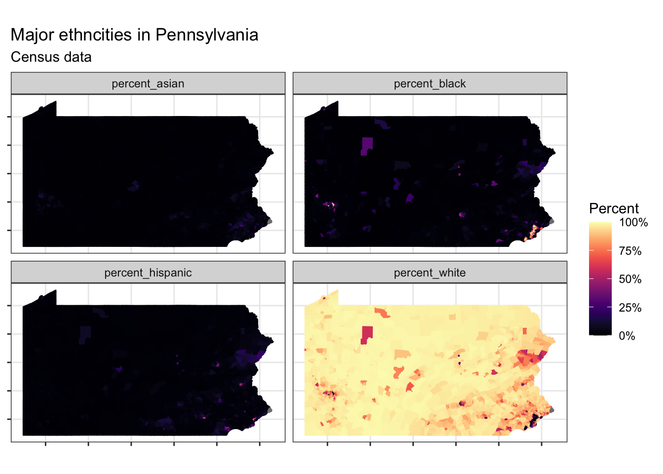
Resources used: