USL in the 538 Global Club Soccer Rankings

This post was originally run with data from August 2018. 538 does not provide historical rankings, so I had to rerun the code with June 2023 data when I migrated my blog.

538 recently added the United Soccer League to their Soccer Power Index ratings. I’m a Riverhounds fan, so I wanted to see how the team compared to teams from leagues around the world.

library(tidyverse)
library(ggrepel)

theme_set(theme_bw())

df <- read_csv("https://projects.fivethirtyeight.com/soccer-api/club/spi_global_rankings.csv", progress = FALSE) %>% 
  group_by(league) %>% 
  mutate(league_spi = median(spi)) %>% 
  ungroup() %>% 
  mutate(league = fct_reorder(league, league_spi))

df

# A tibble: 641 × 8
    rank prev_rank name                     league    off   def   spi league_spi
   <dbl>     <dbl> <chr>                    <fct>   <dbl> <dbl> <dbl>      <dbl>
 1     1         1 Manchester City          Barcla…  2.79  0.28  92         72.8
 2     2         2 Bayern Munich            German…  3.04  0.68  87.7       67.6
 3     3         3 Barcelona                Spanis…  2.45  0.43  86.4       67.0
 4     4         4 Real Madrid              Spanis…  2.56  0.6   84.4       67.0
 5     5         5 Liverpool                Barcla…  2.63  0.67  83.9       72.8
 6     6         6 Arsenal                  Barcla…  2.53  0.61  83.9       72.8
 7     7         7 Newcastle                Barcla…  2.38  0.53  83.7       72.8
 8     8         8 Napoli                   Italy …  2.3   0.51  83.2       63.4
 9     9         9 Borussia Dortmund        German…  2.83  0.84  82.9       67.6
10    10        10 Brighton and Hove Albion Barcla…  2.47  0.73  80.9       72.8
# ℹ 631 more rows

df %>% 
  ggplot(aes(spi, league)) +
  geom_jitter(aes(color = league), show.legend = FALSE,
              height = .2,
              alpha = .7) +
  geom_jitter(data = df %>% filter(name == "Pittsburgh Riverhounds"),
              show.legend = FALSE,
              height = .2,
              alpha = .7) +
  geom_label_repel(data = df %>% filter(name == "Pittsburgh Riverhounds"), 
                   aes(label = name), 
                   size = 3,
                   show.legend = FALSE,
                   force = 6) +
  labs(title = "538 Soccer Power Index",
       subtitle = "One dot = one team",
       y = NULL,
       x = "Soccer Power Index",
       caption = "538 data, @conor_tompkins")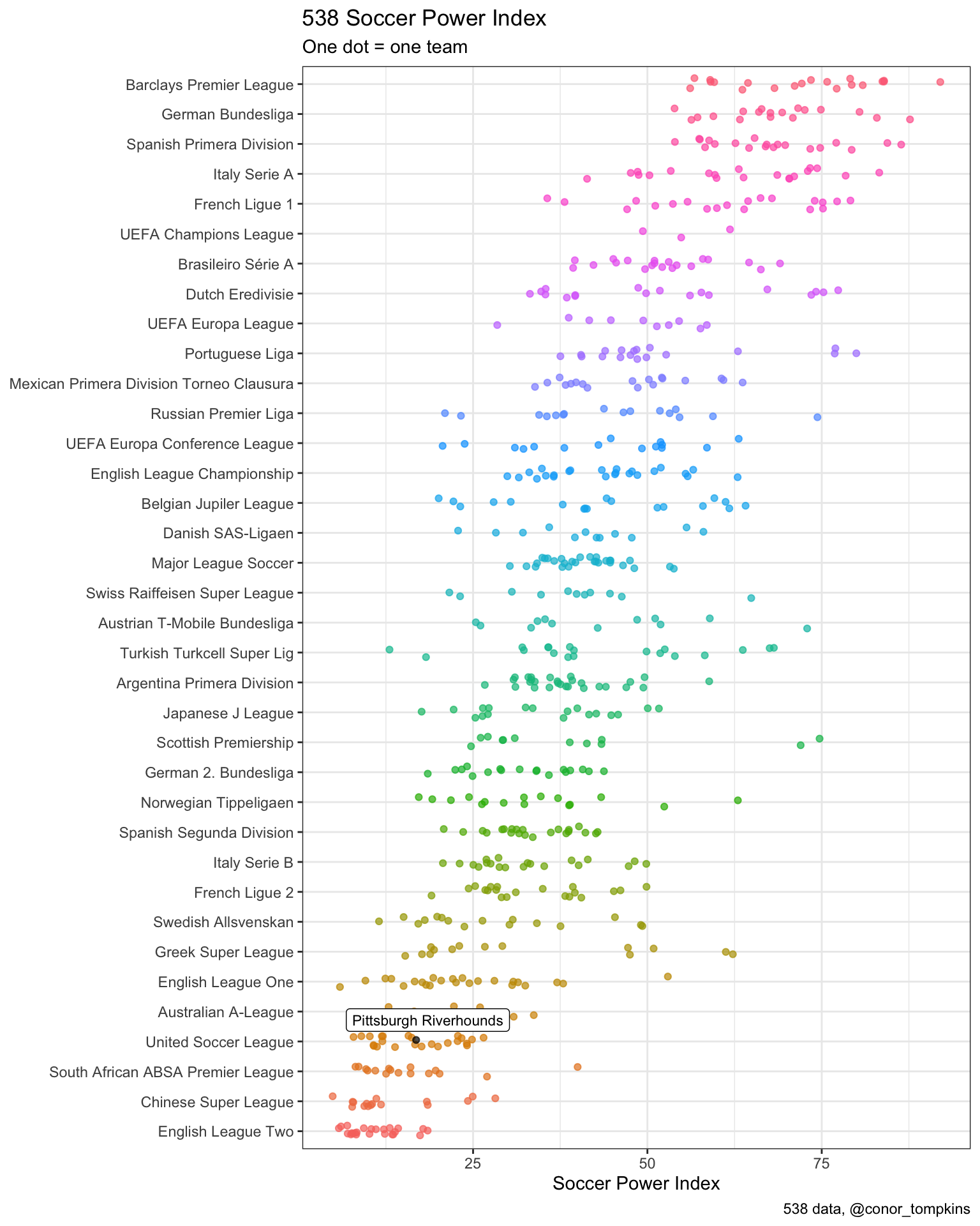

df %>% 
  ggplot(aes(spi, league)) +
  geom_jitter(aes(color = league), show.legend = FALSE,
              height = .2,
              alpha = .7) +
  labs(title = "538 Soccer Power Index",
       subtitle = "One dot = one team",
       y = NULL,
       x = "Soccer Power Index",
       caption = "538 data, @conor_tompkins")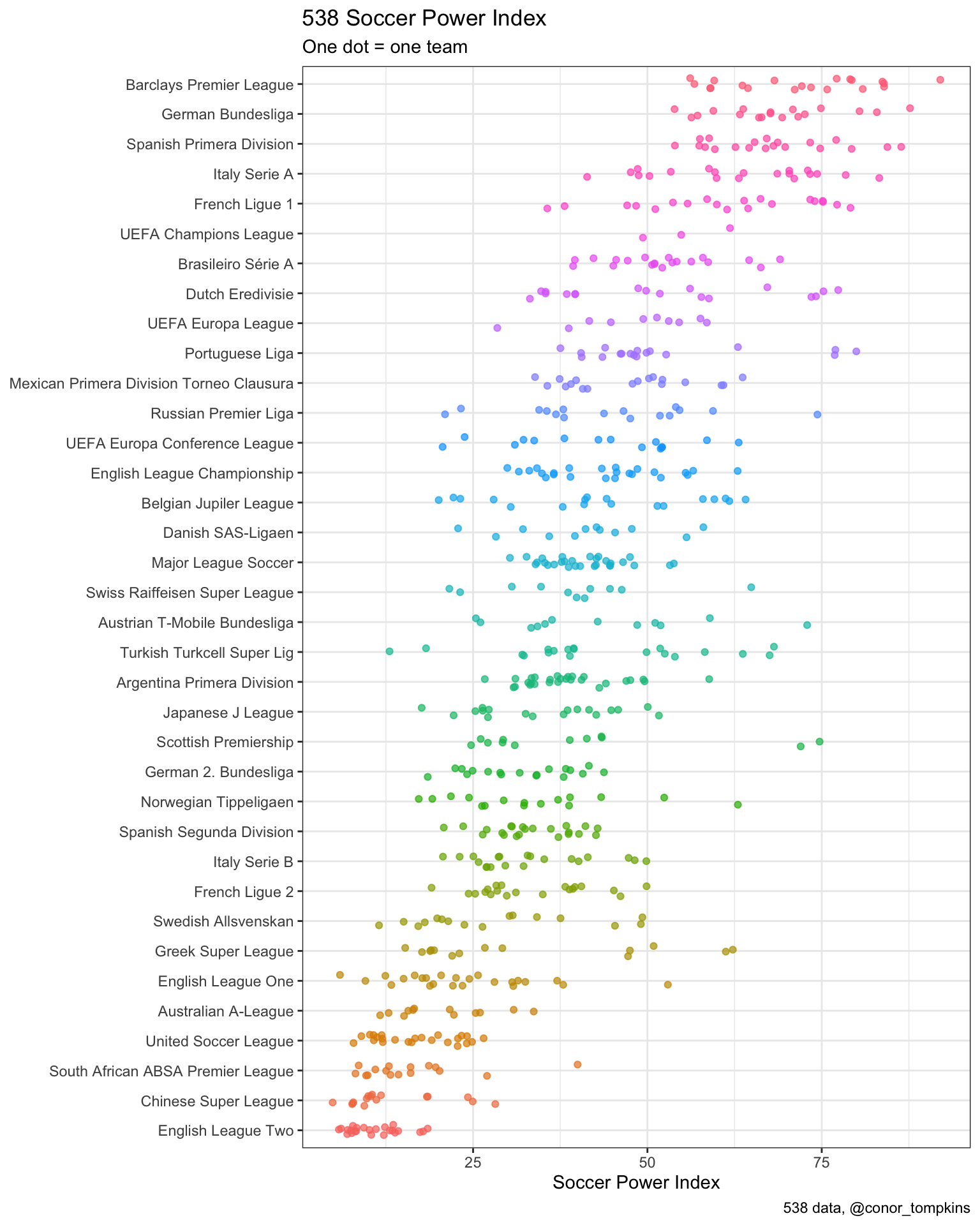

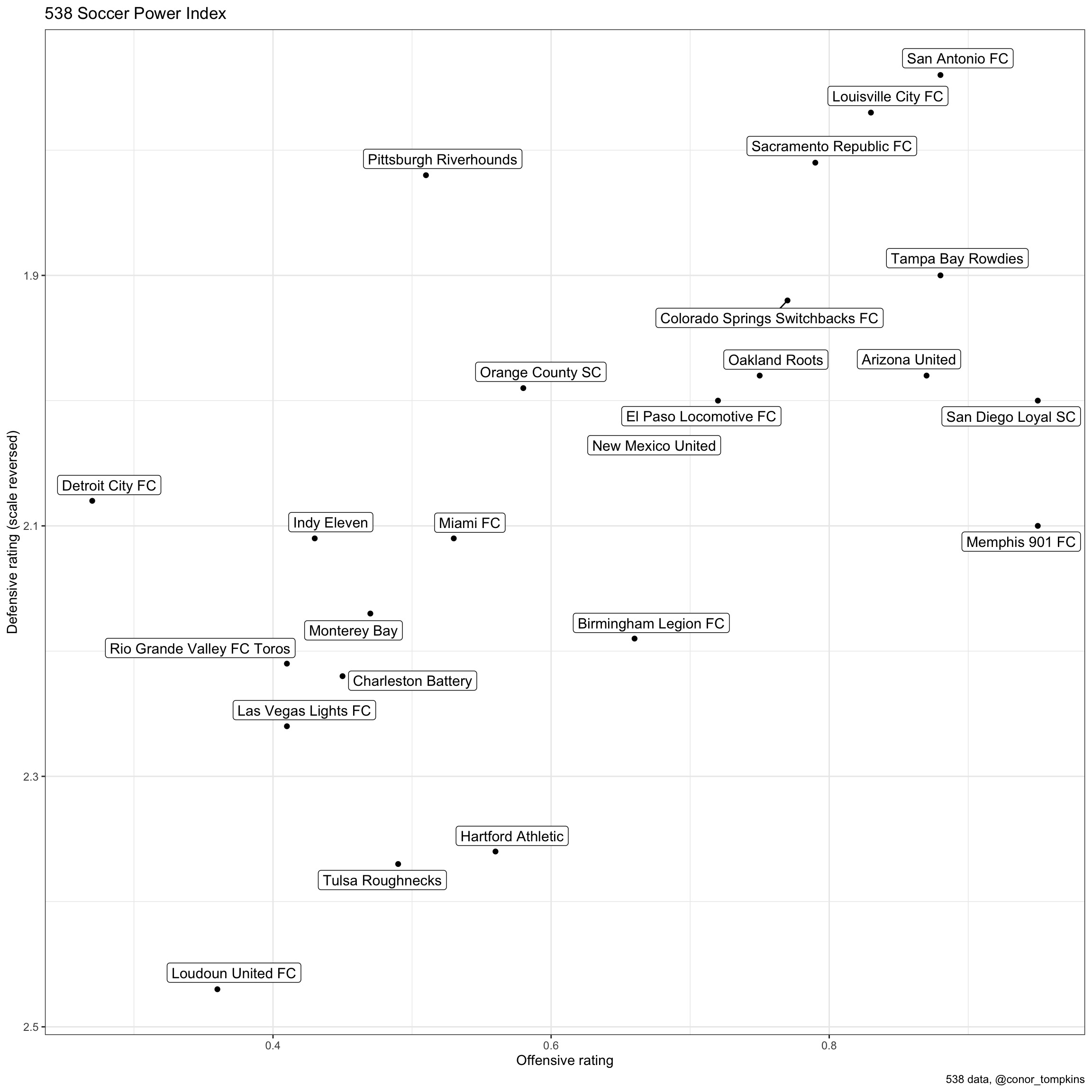
This shows the offensive and defensive ratings of each USL team. The Riverhounds are squarely in the #LilleyBall quadrant.

df %>% 
  filter(league == "United Soccer League") %>% 
  ggplot(aes(off, def, label = name)) +
  geom_point() +
  geom_label_repel(size = 4,
                   force = 4) +
  scale_y_reverse() +
  labs(title = "538 Soccer Power Index",
       y = "Defensive rating (scale reversed)",
       x = "Offensive rating",
       caption = "538 data, @conor_tompkins")