Forecasting US gas prices with Brent Crude Oil

In this post, I analyze the relationship between the Brent Crude oil index (BC) and US gas prices at the pump GASREGW. I use time series forecasting with exogenous variables to test whether BC is a useful predictor of the price of gas in the US.

Setup code:

library(fpp3)
library(tidyverse)
library(fredr)
library(janitor)
library(future)
library(slider)
library(hrbrthemes)
library(tictoc)
library(arrow)
library(tidytext)
library(glue)
library(broom)
library(ggrepel)

toc_quiet <- TRUE

custom_theme <- theme_bw(base_size = 14)

theme_set(custom_theme)

plan(multisession)

options(scipen = 999, digits = 4)

set.seed(1234)

This code pulls the data from FRED.

fred_df_raw <- c(
  "brent_crude" = "DCOILBRENTEU", #brent crude
  "us_consumer_gas" = "GASREGW" #us gas price
) |>
  map_dfr(fredr, .id = "series")

Exploratory data analysis

The results from FRED are stored in a dataframe (series, date, value). Here I clean up the dataframe and filter it so the begining and end of each series align. BC is measured daily, while the US gas price is measured weekly, so I aggregate the data to the year-week level.

oil_prices <- fred_df_raw |>
  select(series, date, value) |>
  rename(price = value)

aligned_time_window <- oil_prices |>
  summarize(start_date = min(date), end_date = max(date), .by = series) |>
  summarize(start_date = max(start_date), end_date = min(end_date))

oil_prices <- oil_prices |>
  filter(between(
    date,
    aligned_time_window$start_date,
    aligned_time_window$end_date
  ))

oil_prices <- oil_prices |>
  mutate(date_week = yearweek(date)) |>
  summarize(price = mean(price, na.rm = TRUE), .by = c(series, date_week)) |>
  arrange(series, date_week) |>
  mutate(flag_imputed_price = is.na(price)) |>
  fill(price, .by = series, .direction = "down")

oil_prices <- as_tsibble(oil_prices, key = series, index = date_week)

has_gaps(oil_prices) |> pull(.gaps) |> any() == FALSE

[1] TRUE

glimpse(oil_prices)

Rows: 3,718
Columns: 4
Key: series [2]
$ series             <chr> "brent_crude", "brent_crude", "brent_crude", "brent…
$ date_week          <week> 1990 W34, 1990 W35, 1990 W36, 1990 W37, 1990 W38, …
$ price              <dbl> 30.48, 27.65, 31.09, 32.01, 35.71, 40.79, 37.64, 40…
$ flag_imputed_price <lgl> FALSE, FALSE, FALSE, FALSE, FALSE, FALSE, FALSE, FA…

This plots the two series in a faceted chart. They follow each other closely.

autoplot(oil_prices) +
  facet_wrap(vars(series), scale = "free_y", ncol = 1) +
  guides(color = "none") +
  scale_y_continuous(label = ~ str_c("$", .x)) +
  labs(x = "Date", y = "Price")

This calculates the week-over-week % change and a % change indexed to the first observation, for each series. The WoW graph shows that the US gas price follows BC, but does not have as extreme highs and lows.

oil_comparison <- oil_prices |>
  as_tibble() |>
  mutate(
    wow_pct_change = (price - lag(price)) / lag(price),
    price_indexed = price / first(price),
    .by = series
  ) |>
  mutate(
    decade = (year(date_week) %/% 10),
    decade = str_c(decade, "0s", sep = "")
  )

oil_comparison |>
  ggplot(aes(x = date_week, y = wow_pct_change, color = series)) +
  geom_line() +
  facet_wrap(vars(decade), scales = "free", ncol = 1) +
  labs(
    title = "Week-over-week % change",
    subtitle = "Brent Crude Oil and US Consumer Gas Price",
    x = "Date",
    y = "% change",
    color = "Series"
  ) +
  scale_y_percent() +
  theme(legend.position = "top")

A basic scatterplot of the WoW % change of the two series shows that there is a positive relationship, but does not show an obvious effect.

compare_wow <- oil_comparison |>
  select(series, date_week, wow_pct_change) |>
  pivot_wider(names_from = series, values_from = wow_pct_change)

compare_wow |>
  ggplot(aes(us_consumer_gas, brent_crude)) +
  geom_point(alpha = .1) +
  geom_smooth(method = "lm") +
  labs(
    title = "Week-over-week % change",
    subtitle = "Brent Crude Oil and US Consumer Gas Price",
    x = "US Consumer Gas Price",
    y = "Brent Crude Oil",
    caption = "Axis ranges are not equal"
  )

lm(us_consumer_gas ~ brent_crude, compare_wow)

Call:
lm(formula = us_consumer_gas ~ brent_crude, data = compare_wow)

Coefficients:
(Intercept)  brent_crude  
   0.000682     0.089863  

This line graph of the indexed % change of each series shows that the two series were tightly coupled in the 2000s and 2020s, but diverged in the 1990s and 2010s.

first_week <- min(oil_prices$date_week)

oil_comparison |>
  ggplot(aes(x = date_week, y = price_indexed, color = series)) +
  geom_line() +
  facet_wrap(vars(decade), scales = "free", ncol = 1) +
  labs(
    title = glue("Price of oil indexed to {first_week}"),
    subtitle = "Brent Crude Oil and US Consumer Gas Price",
    x = "Date",
    y = "Index",
    color = "Series"
  ) +
  scale_y_percent() +
  theme(legend.position = "top")

This code decomposes the series into time series components and plots them. The “remainder” component is what cannot be explained by trend or weekly seasonality.

ts_components <- oil_prices |>
  model(
    stl = STL(
      price ~ season(period = "1 year")
    )
  ) |>
  components() |>
  select(-season_adjust) |>
  rename(weekly_seasonality = `season_1 year`)

ts_components |>
  select(
    series,
    date_week,
    price,
    trend,
    weekly_seasonality,
    remainder
  ) |>
  pivot_longer(-c(series, date_week)) |>
  mutate(
    name = factor(
      name,
      levels = c(
        "price",
        "trend",
        "weekly_seasonality",
        "remainder"
      )
    )
  ) |>
  autoplot() +
  facet_wrap(vars(name, series), scale = "free_y", ncol = 2) +
  guides(color = "none") +
  labs(x = "Date") +
  theme(axis.text.x = element_text(size = 8))

The two series are highly correlated across various decompositions of the time series.

ts_components |>
  select(
    series,
    date_week,
    price,
    trend,
    weekly_seasonality,
    remainder
  ) |>
  pivot_longer(-c(series, date_week)) |>
  pivot_wider(names_from = series, values_from = value) |>
  mutate(
    name = factor(
      name,
      levels = c(
        "price",
        "trend",
        "weekly_seasonality",
        "remainder"
      )
    )
  ) |>
  ggplot(aes(us_consumer_gas, brent_crude)) +
  geom_point(size = .5, alpha = .1) +
  facet_wrap(vars(name), scales = "free")

Modelling US gas price

For cross-validatation, I break the us_consumer_gas series into chunks of 4 years (208 weeks) of each series, stepping forward by 3 years (156 weeks). The chunks overlap each other by 1 year. Then I train various models of different types, which I will then forecast and measure their accuracy to determine which model structure is most appropriate.

us_oil_prices <- oil_prices |>
  filter(date_week >= yearweek("2000 W1")) |>
  filter(series == "us_consumer_gas")

ts_cv <- us_oil_prices |>
  slide_tsibble(.size = cv_size, .step = cv_step)

brent_crude_exo <- oil_prices |>
  filter(series == "brent_crude") |>
  as_tibble() |>
  select(date_week, price) |>
  rename(brent_crude = price) |>
  mutate(
    brent_crude_lag1 = lag(brent_crude, 1),
    brent_crude_lag5 = lag(brent_crude, 5),
    brent_crude_lag10 = lag(brent_crude, 10),
    brent_crude_mean10 = slide_dbl(brent_crude + 1, ~ mean(.x), .before = 10),
    brent_crude_mean30 = slide_dbl(brent_crude + 1, ~ mean(.x), .before = 30),
    brent_crude_mean60 = slide_dbl(brent_crude + 1, ~ mean(.x), .before = 60),
    brent_crude_max10 = slide_dbl(brent_crude + 1, ~ max(.x), .before = 10),
    brent_crude_max20 = slide_dbl(brent_crude + 1, ~ max(.x), .before = 20),
    brent_crude_max30 = slide_dbl(brent_crude + 1, ~ max(.x), .before = 30),
  ) |>
  drop_na()

ts_cv <- left_join(ts_cv, brent_crude_exo)

ts_cv |>
  as_tibble() |>
  summarize(
    start_date = min(date_week),
    end_date = max(date_week),
    .by = .id
  ) |>
  ggplot(aes(x = start_date, xend = end_date, y = .id)) +
  geom_segment() +
  scale_y_reverse() +
  labs(x = "Time window", y = "Cross-validation chunk")

I use log(price + 1) to constrain the forecasts to be positive. I use fourier terms like fourier(365.25 / 7, k = x) to represent the impact of within-year weekly seasonality without having to make ~52 dummy variables. K varies how “smooth” the representation is. Higher values of K fit the model closer to the variance in the data, and lower values of K use a simpler pattern.

tic()
ts_models_benchmark <- ts_cv |>
  model(
    #simple models for benchmarking
    naive = NAIVE(price),
    dcmp = decomposition_model(
      STL(log(price + 1) ~ season(period = "1 year")),
      ETS(season_adjust ~ season("N"))
    ),
    mean_16 = MEAN(price, window(16)),
    mean_52 = MEAN(price, window(52))
  )

ts_models_lm <- ts_cv |>
  model(
    #linear models
    tslm_k1 = TSLM(log(price + 1) ~ fourier(365.25 / 7, K = 1)),
    tslm_k3 = TSLM(log(price + 1) ~ fourier(365.25 / 7, K = 3)),
    tslm_k5 = TSLM(log(price + 1) ~ fourier(365.25 / 7, K = 5)),
    tslm_k7 = TSLM(log(price + 1) ~ fourier(365.25 / 7, K = 7))
  )

ts_models_dhr <- ts_cv |>
  model(
    #dhr means dynamic harmonic regression
    #these ARIMA models constrain the seasonal PDQ
    dhr_k1_pdq = ARIMA(
      log(price + 1) ~ fourier(365.25 / 7, K = 1) +
        PDQ(0, 0, 0)
    ),
    dhr_k3_pdq = ARIMA(
      log(price + 1) ~ fourier(365.25 / 7, K = 3) +
        PDQ(0, 0, 0)
    ),
    dhr_k5_pdq = ARIMA(
      log(price + 1) ~ fourier(365.25 / 7, K = 5) +
        PDQ(0, 0, 0)
    ),
    dhr_k7_pdq = ARIMA(
      log(price + 1) ~ fourier(365.25 / 7, K = 7) +
        PDQ(0, 0, 0)
    ),
    #these ARIMA models let the ARIMA() function search the parameter space for optimal values of P, D, Q
    dhr_k1_free = ARIMA(
      log(price + 1) ~ fourier(365.25 / 7, K = 1)
    ),
    dhr_k3_free = ARIMA(
      log(price + 1) ~ fourier(365.25 / 7, K = 3)
    ),
    dhr_k5_free = ARIMA(
      log(price + 1) ~ fourier(365.25 / 7, K = 5)
    ),
    dhr_k7_free = ARIMA(
      log(price + 1) ~ fourier(365.25 / 7, K = 7)
    )
  )
toc(quiet = toc_quiet)

ts_models_combined <- list(ts_models_benchmark, ts_models_lm, ts_models_dhr) |>
  reduce(left_join, by = join_by(.id, series))

glimpse(ts_models_combined)

Rows: 8
Columns: 18
Key: .id, series [8]
$ .id         <int> 1, 2, 3, 4, 5, 6, 7, 8
$ series      <chr> "us_consumer_gas", "us_consumer_gas", "us_consumer_gas", "…
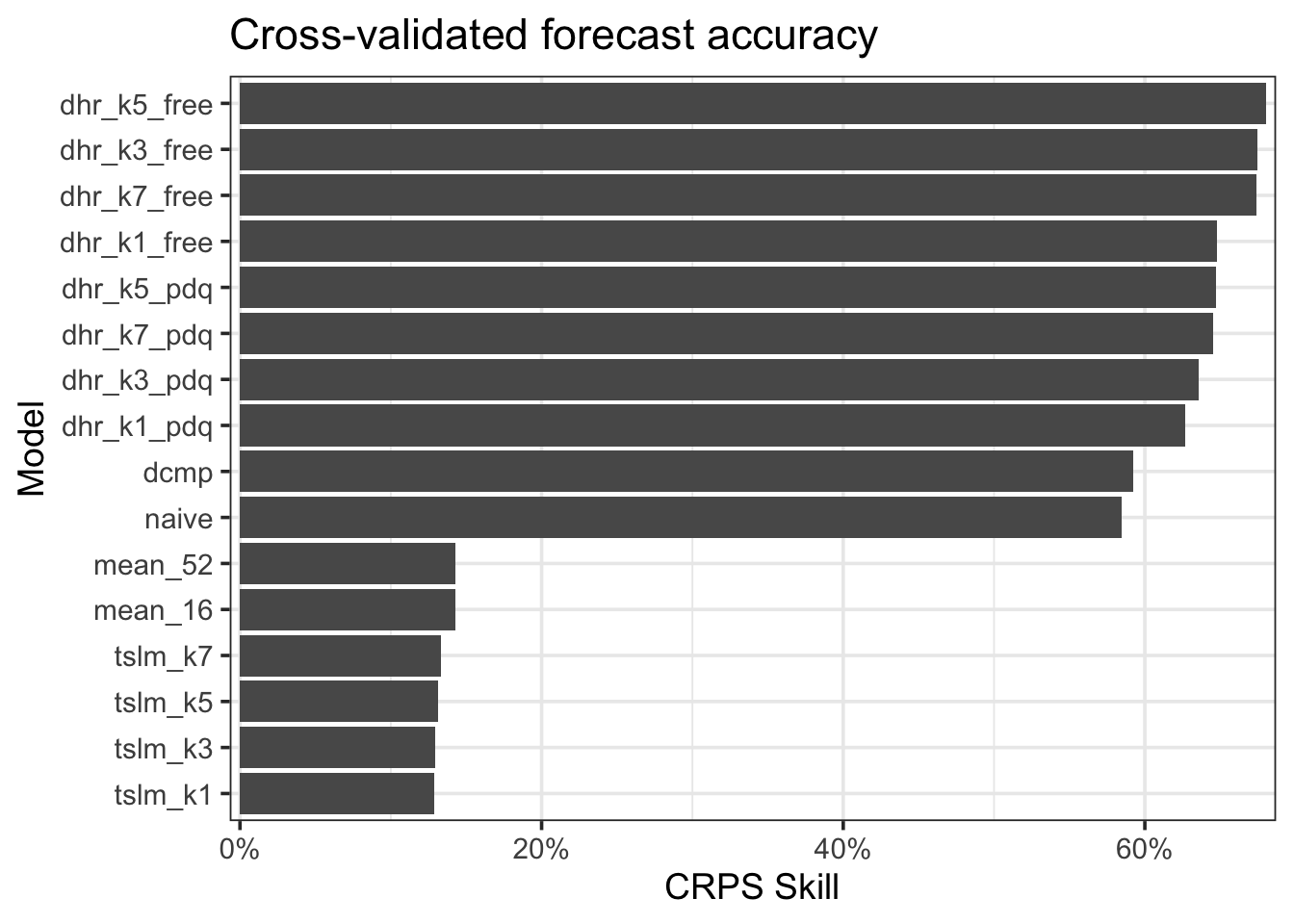
$ naive       <model> [NAIVE], [NAIVE], [NAIVE], [NAIVE], [NAIVE], [NAIVE], [NAI…
$ dcmp        <model> [STL decomposition model], [STL decomposition model], [S…
$ mean_16     <model> [MEAN], [MEAN], [MEAN], [MEAN], [MEAN], [MEAN], [MEAN], …
$ mean_52     <model> [MEAN], [MEAN], [MEAN], [MEAN], [MEAN], [MEAN], [MEAN], …
$ tslm_k1     <model> [TSLM], [TSLM], [TSLM], [TSLM], [TSLM], [TSLM], [TSLM], …
$ tslm_k3     <model> [TSLM], [TSLM], [TSLM], [TSLM], [TSLM], [TSLM], [TSLM], …
$ tslm_k5     <model> [TSLM], [TSLM], [TSLM], [TSLM], [TSLM], [TSLM], [TSLM], …
$ tslm_k7     <model> [TSLM], [TSLM], [TSLM], [TSLM], [TSLM], [TSLM], [TSLM], …
$ dhr_k1_pdq  <model> [LM w/ ARIMA(2,1,2) errors], [LM w/ ARIMA(1,1,0) errors]…
$ dhr_k3_pdq  <model> [LM w/ ARIMA(2,1,1) errors], [LM w/ ARIMA(0,1,1) errors]…
$ dhr_k5_pdq  <model> [LM w/ ARIMA(1,1,0) errors], [LM w/ ARIMA(0,1,1) errors]…
$ dhr_k7_pdq  <model> [LM w/ ARIMA(1,1,0) errors], [LM w/ ARIMA(0,1,1) errors]…
$ dhr_k1_free <model> [LM w/ ARIMA(4,1,1)(1,0,0)[52] errors], [LM w/ ARIMA(1,1…
$ dhr_k3_free <model> [LM w/ ARIMA(2,1,1)(1,0,0)[52] errors], [LM w/ ARIMA(0,1…
$ dhr_k5_free <model> [LM w/ ARIMA(1,1,0) errors], [LM w/ ARIMA(0,1,1) errors]…
$ dhr_k7_free <model> [LM w/ ARIMA(2,1,1)(1,0,0)[52] errors], [LM w/ ARIMA(0,1…

Once the models are trained, I forecast 52 weeks ahead.

tic()
test_fc <- ts_models_combined |>
  forecast(h = 52)
toc(quiet = toc_quiet)

Then I calculate the accuracy of those forecasts. I calculate the root mean squared error and the “skill score” of CRPS (continuous ranked probability score). CRPS measures how well the forecast distribution fits the observed data, and skill_score() compares that to the CRPS of a naive model. Think of crps_skill like the % improvement over a benchmark model.

tic()
test_acc <- accuracy(
  test_fc,
  oil_prices,
  list(rmse = RMSE, crps_skill = skill_score(CRPS))
) |>
  arrange(series, desc(crps_skill))
toc(quiet = toc_quiet)

test_acc |>
  mutate(
    .model = reorder_within(
      x = .model,
      by = crps_skill,
      within = series
    )
  ) |>
  ggplot(aes(x = crps_skill, y = .model)) +
  geom_col() +
  scale_x_percent() +
  scale_y_reordered() +
  labs(
    title = "Cross-validated forecast accuracy",
    x = "CRPS Skill",
    y = "Model"
  )

The dynamic harmonic regression models (dhr) clearly outperform all the other models.

Finding the horizon

Based on the cross-validated accuracy, the dhr5_free did the best. This code calculates the accuracy of dhr5_free and the best benchmark model dcmp at each index of the forecast horizon.

final_models <- ts_cv |>
  model(
    dcmp = decomposition_model(
      STL(log(price + 1) ~ season(period = "1 year")),
      ETS(season_adjust ~ season("N"))
    ),
    dhr_k5_free = ARIMA(
      log(price + 1) ~ fourier(365.25 / 7, K = 5)
    )
  )

# 4. Add horizon index
fc_h <- final_models |>
  forecast(h = 52) |>
  group_by(.id, .model) |>
  mutate(h = row_number()) |>
  ungroup() |>
  as_fable(response = "price", distribution = price)

# 5. Accuracy by horizon
acc_by_h <- accuracy(fc_h, oil_prices, by = c("h", ".model")) # one row per horizon & model

acc_by_h |>
  ggplot(aes(x = h, y = RMSE, color = .model)) +
  geom_vline(xintercept = 12, lty = 2) +
  geom_line() +
  labs(
    title = "Avg. forecast error across forecast horizon",
    x = "Forecast horizon (weeks)",
    y = "Error (RMSE)",
    color = "Model"
  ) +
  scale_y_continuous(label = \(x) str_c("$", x)) +
  theme(legend.position = "top")

#Accuracy by horizon and .id
acc_by_h_id <- fc_h |>
  as_tibble() |>
  rename(price_fc = price) |>
  left_join(
    oil_prices |>
      as_tibble() |>
      rename(price_actual = price),
    by = c("series", "date_week")
  ) |>
  mutate(
    error = price_actual - price_fc,
    abs_err = abs(error),
    ape = abs_err / price_actual # fractional (0–1); *100 for %
  ) |>
  group_by(.model, .id, h) |>
  summarise(
    RMSE = sqrt(mean(error^2, na.rm = TRUE)),
    .groups = "drop"
  )

Breaking the error graph out by cross-validation .id shows a similar pattern.

acc_percentiles <- acc_by_h_id |>
  select(.id, h, .model, RMSE) |>
  group_by(.model, h) |>
  reframe(
    quants = quantile(RMSE, probs = c(.1, .25, .5, .75, .95)),
    quant_labs = c("10%", "25%", "50%", "75%", "90%")
  ) |>
  pivot_wider(names_from = quant_labs, values_from = quants)

acc_percentiles |>
  ggplot(aes(x = h, color = .model)) +
  geom_ribbon(
    aes(ymin = `10%`, ymax = `90%`, fill = .model),
    alpha = 0.2,
    lwd = .1
  ) +
  geom_ribbon(
    aes(ymin = `25%`, ymax = `75%`, fill = .model),
    alpha = 0.4,
    lwd = .1
  ) +
  geom_line(aes(y = `50%`), linewidth = 0.8) +
  geom_vline(xintercept = 12, lty = 2) +
  labs(
    title = "Forecast error (RMSE) across forecast horizon",
    subtitle = "Median and 10/25/75/90th percentiles by forecast horizon",
    x = "Forecast horizon (weeks)",
    y = "RMSE"
  ) +
  guides(fill = "none", color = "none") +
  scale_y_continuous(labels = \(x) str_c("$", x)) +
  theme(legend.position = "top")

The two models have similar error trajectories over the first 8 weeks, but significantly diverage over the next ~25 weeks. The error for dcmp increases much more rapidly than dhr5_free. dhr5_free also has much lower error variance. Based on RMSE, 12 weeks is a reasonable forecast horizon for dhr5_free.

Interestingly, the error curve for dcmp continues to increase after week ~20, while dhr5_free stabilizes. Then the error curve for dcmp decreases after week ~32. The variance in the error of both models increases, as indicated by the wider interquartile range in the line graph. This variance is driven by outliers from one cross-validation forecast. Further cross-validation could help smooth that out, but I don’t have the compute power for that at hand.

My hypothesis for this is that in the short-term, the US gas price is driven by events, but long-term variance is driven by the global oil market, the push and pull of supply and demand, and long-term structural aspects of the global economy. It may be easier for a model without exogenous variables to forecast what the price of oil will be in 52 weeks than in 32 weeks.

Forecasting with Brent Crude Oil as exogenous predictor

Next I train additional models based on dhr5_free that consider various transformation of Brent Crude (BC) as exogenous predictors, in addition to the US gas price time series itself. The choices in these transformations are somewhat arbitrary, and could be tested more rigorously.

• Models with bc_lag at the end use a weekly lag of BC as a predictor. “lag1” means that it uses last week’s BC to predict this week’s US gas price.
• Models with bc_mean at the end use a trailing rolling average of BC as an predictor. “mean10” means that it uses a 10 week trailing rolling average of BC to predict this week’s US gas price.
• Models with bc_max at the end use a trailing rolling maximum of BC as an predictor. “max10” means that it uses a 10 week trailing rolling high of BC to predict this week’s US gas price.

tic()
models_cv_benchmark <- ts_cv |>
  model(
    dcmp = decomposition_model(
      STL(log(price + 1) ~ season(period = "1 year")),
      ETS(season_adjust ~ season("N"))
    ),
    dhr_k5_free = ARIMA(
      log(price + 1) ~ fourier(365.25 / 7, K = 5)
    )
  )

models_cv_exo <- ts_cv |>
  model(
    dhr_k5_free_bc_lag0 = ARIMA(
      log(price + 1) ~ fourier(365.25 / 7, K = 5) +
        brent_crude
    ),
    dhr_k5_free_bc_lag1 = ARIMA(
      log(price + 1) ~ fourier(365.25 / 7, K = 5) +
        brent_crude_lag1
    ),
    dhr_k5_free_bc_lag5 = ARIMA(
      log(price + 1) ~ fourier(365.25 / 7, K = 5) +
        brent_crude_lag5
    ),
    dhr_k5_free_bc_lag10 = ARIMA(
      log(price + 1) ~ fourier(365.25 / 7, K = 5) +
        brent_crude_lag10
    ),
    dhr_k5_free_bc_mean10 = ARIMA(
      log(price + 1) ~ fourier(365.25 / 7, K = 5) +
        brent_crude_mean10
    ),
    dhr_k5_free_bc_mean30 = ARIMA(
      log(price + 1) ~ fourier(365.25 / 7, K = 5) +
        brent_crude_mean30
    ),
    dhr_k5_free_bc_mean60 = ARIMA(
      log(price + 1) ~ fourier(365.25 / 7, K = 5) +
        brent_crude_mean60
    ),
    dhr_k5_free_bc_max10 = ARIMA(
      log(price + 1) ~ fourier(365.25 / 7, K = 5) +
        brent_crude_max10
    ),
    dhr_k5_free_bc_max20 = ARIMA(
      log(price + 1) ~ fourier(365.25 / 7, K = 5) +
        brent_crude_max20
    ),
    dhr_k5_free_bc_max30 = ARIMA(
      log(price + 1) ~ fourier(365.25 / 7, K = 5) +
        brent_crude_max30
    )
  )

models_cv_all <- left_join(
  models_cv_benchmark,
  models_cv_exo,
  by = join_by(.id, series)
)
toc(quiet = toc_quiet)

glimpse(models_cv_all)

Rows: 8
Columns: 14
Key: .id, series [8]
$ .id                   <int> 1, 2, 3, 4, 5, 6, 7, 8
$ series                <chr> "us_consumer_gas", "us_consumer_gas", "us_consum…
$ dcmp                  <model> [STL decomposition model], [STL decomposition mo…
$ dhr_k5_free           <model> [LM w/ ARIMA(1,1,0) errors], [LM w/ ARIMA(0,1,…
$ dhr_k5_free_bc_lag0   <model> [LM w/ ARIMA(3,0,1)(1,0,0)[52] errors], [LM w/…
$ dhr_k5_free_bc_lag1   <model> [LM w/ ARIMA(3,0,0)(1,0,0)[52] errors], [LM w/…
$ dhr_k5_free_bc_lag5   <model> [LM w/ ARIMA(2,0,0) errors], [LM w/ ARIMA(2,0,…
$ dhr_k5_free_bc_lag10  <model> [LM w/ ARIMA(2,0,0) errors], [LM w/ ARIMA(2,0,…
$ dhr_k5_free_bc_mean10 <model> [LM w/ ARIMA(3,0,1)(1,0,0)[52] errors], [LM w/…
$ dhr_k5_free_bc_mean30 <model> [LM w/ ARIMA(2,0,0) errors], [LM w/ ARIMA(2,0,…
$ dhr_k5_free_bc_mean60 <model> [LM w/ ARIMA(1,1,0) errors], [LM w/ ARIMA(2,0,…
$ dhr_k5_free_bc_max10  <model> [LM w/ ARIMA(1,1,0) errors], [LM w/ ARIMA(1,0,…
$ dhr_k5_free_bc_max20  <model> [LM w/ ARIMA(2,0,0) errors], [LM w/ ARIMA(1,0,…
$ dhr_k5_free_bc_max30  <model> [LM w/ ARIMA(2,1,1)(1,0,0)[52] errors], [LM w/…

Next I forecast the models 12 weeks ahead and find the accuracy.

horizon_data <- new_data(ts_cv, 12) |>
  left_join(brent_crude_exo, by = "date_week")

tic()
cv_fc <- forecast(models_cv_all, horizon_data)
toc(quiet = toc_quiet)

tic()
cv_acc <- accuracy(
  cv_fc,
  oil_prices,
  list(rmse = RMSE, crps_skill = skill_score(CRPS))
) |>
  arrange(desc(crps_skill))
toc(quiet = toc_quiet)

The model (dhr_k5_free_bc_mean10) that uses a 10-week moving average of BC as a predictor has the best crps_skill. dhr_k5_free_bc_mean10 provides a ~5 percentage point increase in accuracy over the “vanilla” dhr_k5_free model, while most of the other models with exogenous variables do worse than dhr_k5_free. This shows that the relationship between the price of gas in the US and BC is not straightforward.

cv_acc |>
  mutate(.model = fct_reorder(.model, crps_skill)) |>
  ggplot(aes(crps_skill, .model)) +
  geom_col() +
  scale_x_percent() +
  scale_y_reordered() +
  coord_cartesian(xlim = c(.8, .95)) +
  labs(
    title = "Cross-validated forecast accuracy",
    subtitle = "US Consumer Gas Price",
    x = "CRPS Skill",
    y = "Model"
  )

cv_acc |>
  ggplot(aes(crps_skill, rmse)) +
  geom_point() +
  geom_label_repel(aes(label = .model)) +
  scale_x_percent() +
  scale_y_reverse(label = \(x) str_c("$", x)) +
  labs(
    title = "Cross-validated forecast accuracy",
    subtitle = "US Consumer Gas Price",
    caption = "Y axis reversed",
    x = "CRPS Skill",
    y = "RMSE ($)"
  )

This shows the last cross-validation forecast of the best model (dhr_k5_free_bc_mean10). The average (indicated by the blue line) closely follows the observed data (black line), and the observed data do not fall outside the prediction intervals. This reinforces that the model performs well in terms of CRPS skill score.

fc_window <- cv_fc |>
  filter(.model == best_model, .id == max(.id)) |>
  distinct(date_week)

cv_fc |>
  filter(.model == best_model, .id == max(.id)) |>
  autoplot() +
  autolayer(us_oil_prices |> semi_join(fc_window)) +
  facet_wrap(vars(.model)) +
  scale_y_continuous(label = \(x) str_c("$", x)) +
  guides(fill_ramp = guide_legend(title = "Prediction interval")) +
  labs(
    title = "Last cross-validation forecast",
    subtitle = "Black line shows actual price",
    x = "Date",
    y = "Price"
  ) +
  theme(
    legend.position = "bottom"
  )

Scenario forecasts

Finally, I refit dhr_k5_free_bc_mean10 against the entire training set. The following chart shows the estimate for each term in the model. Even though the estimate for brent_crude_mean10 is relatively lower than the other terms, the cross-validation results show that it is a meaningful variable in terms of predictive power.

ts_train_final <- oil_prices |>
  filter(date_week >= yearweek("2000 W1")) |>
  filter(series == "us_consumer_gas") |>
  left_join(brent_crude_exo, by = join_by(date_week))

ts_model_final <- ts_train_final |>
  model(
    dhr_k5_free_bc_mean10 = ARIMA(
      log(price + 1) ~ fourier(365.25 / 7, K = 5) +
        brent_crude_mean10
    )
  )

model_terms <- ts_model_final |>
  tidy() |>
  select(term, estimate) |>
  mutate(estimate = round(estimate, 4))

model_terms |>
  mutate(term = fct_reorder(term, estimate)) |>
  ggplot(aes(x = estimate, y = term)) +
  geom_col()

Then I set up some future scenarios of Brent Crude (BC) to use as predictors for a true forecast. I create the following 12-week scenarios:

• 20% decrease in BC price over 12 weeks
• BC stabilizes at the current price
• 20% increase in BC price over 12 weeks

final_fc_h <- 12

generate_horizon_exo <- function(x, price_vec) {
  horizon <- new_data(x, n = final_fc_h) |>
    mutate(brent_crude = price_vec)

  bind_rows(x, horizon) |>
    mutate(
      brent_crude_mean10 = slide_dbl(brent_crude + 1, ~ mean(.x), .before = 10)
    ) |>
    slice_tail(n = final_fc_h)
}

last_price <- oil_prices |>
  filter(date_week == max(date_week), series == "brent_crude") |>
  pull(price)

scenario_names <- c(
  glue("20% decrease to ${round(last_price * .8, 2)}"),
  glue("Stabilize at ${round(last_price, 2)}"),
  glue("20% increase to ${round(last_price * 1.2, 2)}")
)

exo_scenarios <- scenarios(
  generate_horizon_exo(
    ts_train_final,
    seq(last_price, last_price * .8, length.out = final_fc_h)
  ),
  generate_horizon_exo(
    ts_train_final,
    rep(last_price, final_fc_h)
  ),
  generate_horizon_exo(
    ts_train_final,
    seq(last_price, last_price * 1.2, length.out = final_fc_h)
  )
) |>
  set_names(scenario_names)

scenario_fc <- ts_model_final |>
  forecast(exo_scenarios) |>
  mutate(
    .scenario = fct_relevel(
      .scenario,
      scenario_names
    )
  ) |>
  select(.scenario, .model, series, price, .mean) |>
  mutate(
    intervals = hilo(price, 80),
    price_lower = intervals$lower,
    price_upper = intervals$upper
  )

legend_text <- "Brent Crude Oil scenario"

ggplot() +
  geom_line(
    data = ts_train_final |>
      slice_tail(n = 52 * .5),
    aes(x = date_week, y = price, colour = "History"),
    color = "black"
  ) +
  geom_ribbon(
    data = scenario_fc,
    aes(
      x = date_week,
      ymin = price_lower,
      ymax = price_upper,
      fill = .scenario
    ),
    alpha = .3
  ) +
  geom_line(
    data = scenario_fc,
    aes(x = date_week, y = .mean, colour = .scenario)
  ) +
  labs(
    title = glue("{final_fc_h} week forecast of US gas price at the pump"),
    subtitle = "Shaded area shows upper and lower bounds of forecast range",
    x = "Date",
    y = "Price",
    fill = legend_text,
    color = legend_text
  ) +
  scale_x_yearweek(
    date_breaks = "6 weeks"
  ) +
  scale_y_continuous(label = \(x) str_c("$", x)) +
  theme(
    legend.position = "bottom",
    legend.title.position = "top"
  )

This model forecasts that the US gas price will increase for the next ~7 weeks regardless of the scenario. The high end of the “Increase” scenario is > $5.50. Prices remain above $4 per gallon in the average outcome for all scenarios. This is likely because the global oil supply chain has already been severely constrained, and even in a best case scenario it would take weeks for oil to transit from its origin to consumer markets.

Future extension

A possible improvement on this method is to include the release of oil from the IEA (International Energy Agency) oil reserves as a term in the model. Oil is released from these reserves to reduce pressure on supply, which should decrease the price. This function is probably similar to a stock market circuit-breaker or time-outs in basketball.