Exploring long-term Pittsburgh weather data

Intro

In this post I will explore the long-term weather history of Pittsburgh. I use {openmeteo} to access the Open-Meteo free weather API to pull weather variables. My intent for this post is to analyze the patterns within the data and practice exploratory data analysis.

My approach is to select a representative sample of the weather variables to reduce redundancy while conserving signal, apply PCA to the remaining variables, and examine the results.

Pull data

These are the weather variables available from the API. I use the “ERA5” model, which uses reanalysis to infer the weather data for older periods of time.

weather_variables()$daily_history_vars

 [1] "weather_code"                      "temperature_2m_mean"              
 [3] "temperature_2m_max"                "temperature_2m_min"               
 [5] "apparent_temperature_mean"         "apparent_temperature_max"         
 [7] "apparent_temperature_min"          "sunrise"                          
 [9] "sunset"                            "daylight_duration"                
[11] "sunshine_duration"                 "precipitation_sum"                
[13] "rain_sum"                          "snowfall_sum"                     
[15] "precipitation_hours"               "wind_speed_10m_max"               
[17] "wind_gusts_10m_max"                "wind_direction_10m_dominant"      
[19] "shortwave_radiation_sum"           "et0_fao_evapotranspiration"       
[21] "cloud_cover_mean"                  "dew_point_2m_mean"                
[23] "dew_point_2m_max"                  "dew_point_2m_min"                 
[25] "relative_humidity_2m_mean"         "relative_humidity_2m_max"         
[27] "relative_humidity_2m_min"          "pressure_msl_mean"                
[29] "wind_speed_10m_mean"               "wet_bulb_temperature_2m_mean"     
[31] "vapour_pressure_deficit_max"       "soil_moisture_0_to_7cm_mean"      
[33] "soil_moisture_7_to_28cm_mean"      "soil_moisture_28_to_100cm_mean"   
[35] "soil_moisture_0_to_100cm_mean"     "soil_temperature_0_to_7cm_mean"   
[37] "soil_temperature_7_to_28cm_mean"   "soil_temperature_28_to_100cm_mean"

There is a download limit on the API, so I wrote a function to download the results and save it to parquet. Since I expected to hit the API limit, the function checks if the file for that decade has already been downloaded, and skips those decades. I ran into some issues with missing data, so I also downloaded a sample of the data to check for missingness before fetching the complete dataset.

# pull ERA5 model reanalysis
#https://open-meteo.com/en/docs/historical-weather-api

#https://archive-api.open-meteo.com/v1/archive?latitude=52.52&longitude=13.41&start_date=2026-09-12&end_date=2026-09-26&daily=temperature_2m_mean&hourly=temperature_2m&models=era5

#https://archive-api.open-meteo.com/v1/archive?latitude=40.44&longitude=-79.99&start_date=1940-01-01&end_date=1940-01-31&daily=temperature_2m_mean&models=era5

# set up the timeframe I want to pull data for

my_location <- "Pittsburgh, PA"

year_start <- 1940

year_end <- 2020

date_target_year <- tibble(
  my_location = my_location,
  year = seq(year_start, year_end, by = 1),
  start = glue("{year}-01-01") |> ymd(),
  end = start
)

# define function to pull a sample of the data from the Open-Meteo API
get_weather_data_test <- function(start, end) {
  filename <- glue(
    "/Users/conorotompkins/Documents/github_repos/ctompkins_quarto_blog/posts/pittsburgh_weather_pca/post_data/era5/test/test_era5_{start}.parquet"
  )

  if (file.exists(filename)) {
    print(glue("{filename} exists"))
  } else {
    print(glue("Fetching weather for {start} to {end}"))

    weather_history(
      location = "Pittsburgh, PA",
      start = start,
      end = end,
      daily = weather_variables()$daily_history_vars,
      model = "era5"
    ) |>
      write_parquet(
        filename
      )
  }
}

pwalk(
  .l = list(date_target_year$start, date_target_year$end),
  .f = get_weather_data_test
)

vars_missing <- open_dataset(
  "/Users/conorotompkins/Documents/github_repos/ctompkins_quarto_blog/posts/pittsburgh_weather_pca/post_data/era5/test"
) |>
  collect() |>
  pivot_longer(cols = -date, values_transform = as.character)

vars_missing |>
  summarize(pct_missing = mean(is.na(value)), .by = c(date)) |>
  filter(pct_missing != 0)

# A tibble: 1 × 2
  date       pct_missing
  <date>           <dbl>
1 1940-01-01       0.158

1940-01-01 is missing data, so I will pull data starting in 1941. I split the API calls by decade to work with the API limit.

year_start <- 1940

date_target_decade <- tibble(
  my_location = my_location,
  decade = seq(year_start, year_end, by = 10),
  start = glue("{decade}-01-01") |> ymd(),
  end = glue("{decade + 9}-12-31") |> ymd()
) |>
  mutate(
    start = case_when(start == min(start) ~ ymd("1941-01-01"), .default = end),
    end = case_when(end == max(end) ~ Sys.Date() - days(1), .default = end)
  )

date_target_decade

weather_history_safe <- safely(.f = weather_history, quiet = FALSE)

weather_history_safe <- slowly(
  weather_history_safe,
  rate = rate_delay(pause = 10 * 6)
)

get_weather_data <- function(location, decade, start, end) {
  filename <- glue(
    "/Users/conorotompkins/Documents/github_repos/ctompkins_quarto_blog/posts/pittsburgh_weather_pca/post_data/era5/weather_data_{decade}.parquet"
  )

  if (file.exists(filename)) {
    print(glue("{filename} exists"))
  } else {
    print(glue("Fetching weather for {location} {start} to {end}"))

    x <- weather_history_safe(
      location = location,
      start = start,
      end = end,
      daily = weather_variables()$daily_history_vars,
      model = "era5"
    )

    if (is.null(x$error)) {
      x$result |>
        mutate(location = location, .before = 1) |>
        write_parquet(filename)
    } else {
      print(x$error)
    }
  }
}

pwalk(
  .l = list(
    date_target_decade$my_location,
    date_target_decade$decade,
    date_target_decade$start,
    date_target_decade$end
  ),
  .f = get_weather_data
)

Once I read the data back from parquet, I get a dataframe with the weather variables from the API. I also calculate some additional date variables that I will use later on.

weather_files <- list.files(
  "/Users/conorotompkins/Documents/github_repos/ctompkins_quarto_blog/posts/pittsburgh_weather_pca/post_data/era5",
  full.names = TRUE,
  pattern = ".parquet"
)

weather_data <- open_dataset(
  weather_files
) |>
  collect() |>
  mutate(
    decade = year(date) %/% 10,
    decade = str_c(decade, "0s"),
    year = year(date),
    yday = yday(date),
    month = month(date, label = TRUE, abbr = TRUE),
    mday = mday(date)
  ) |>
  mutate(location = "Pittsburgh, PA", .before = 1) |>
  select(location, date, decade, year, month, yday, mday, everything())

glimpse(weather_data)

Rows: 31,318
Columns: 45
$ location                                <chr> "Pittsburgh, PA", "Pittsburgh,…
$ date                                    <date> 1941-01-01, 1941-01-02, 1941-…
$ decade                                  <chr> "1940s", "1940s", "1940s", "19…
$ year                                    <dbl> 1941, 1941, 1941, 1941, 1941, …
$ month                                   <ord> Jan, Jan, Jan, Jan, Jan, Jan, …
$ yday                                    <dbl> 1, 2, 3, 4, 5, 6, 7, 8, 9, 10,…
$ mday                                    <int> 1, 2, 3, 4, 5, 6, 7, 8, 9, 10,…
$ daily_weather_code                      <int> 51, 61, 51, 73, 3, 3, 3, 3, 71…
$ daily_temperature_2m_mean               <dbl> 1.4, 5.4, 1.5, -2.6, -6.4, -4.…
$ daily_temperature_2m_max                <dbl> 6.3, 9.7, 4.6, 0.4, -4.8, -1.2…
$ daily_temperature_2m_min                <dbl> -1.7, 2.4, -1.2, -6.5, -8.9, -…
$ daily_apparent_temperature_mean         <dbl> -2.4, 2.1, -1.8, -8.2, -12.6, …
$ daily_apparent_temperature_max          <dbl> 2.4, 7.6, 1.6, -4.8, -10.7, -5…
$ daily_apparent_temperature_min          <dbl> -5.1, -2.0, -4.9, -13.4, -15.0…
$ daily_sunrise                           <chr> "1941-01-01T08:43", "1941-01-0…
$ daily_sunset                            <chr> "1941-01-01T18:04", "1941-01-0…
$ daily_daylight_duration                 <dbl> 33646, 33692, 33741, 33795, 33…
$ daily_sunshine_duration                 <dbl> 30532, 0, 9913, 25200, 15570, …
$ daily_precipitation_sum                 <dbl> 0.2, 8.3, 0.1, 1.3, 0.0, 0.0, …
$ daily_rain_sum                          <dbl> 0.2, 8.3, 0.1, 0.0, 0.0, 0.0, …
$ daily_snowfall_sum                      <dbl> 0.00, 0.00, 0.00, 0.91, 0.00, …
$ daily_precipitation_hours               <dbl> 2, 17, 1, 3, 0, 0, 0, 0, 9, 0,…
$ daily_wind_speed_10m_max                <dbl> 13.5, 15.6, 11.3, 25.9, 21.3, …
$ daily_wind_gusts_10m_max                <dbl> 24.5, 33.1, 20.5, 57.6, 49.7, …
$ daily_wind_direction_10m_dominant       <int> 60, 156, 279, 255, 276, 302, 2…
$ daily_shortwave_radiation_sum           <dbl> 7.07, 0.92, 4.80, 6.17, 5.25, …
$ daily_et0_fao_evapotranspiration        <dbl> 0.98, 0.42, 0.57, 1.00, 0.98, …
$ daily_cloud_cover_mean                  <int> 73, 99, 70, 52, 72, 46, 43, 40…
$ daily_dew_point_2m_mean                 <dbl> -3.4, 3.3, -1.0, -9.3, -14.5, …
$ daily_dew_point_2m_max                  <dbl> -1.5, 9.4, 4.4, -3.7, -11.1, -…
$ daily_dew_point_2m_min                  <dbl> -4.1, -3.4, -3.3, -17.0, -16.8…
$ daily_relative_humidity_2m_mean         <int> 71, 87, 84, 61, 53, 66, 58, 51…
$ daily_relative_humidity_2m_max          <int> 86, 100, 99, 82, 66, 80, 83, 7…
$ daily_relative_humidity_2m_min          <int> 50, 65, 68, 43, 44, 47, 27, 24…
$ daily_pressure_msl_mean                 <dbl> 1028, 1017, 1016, 1011, 1023, …
$ daily_wind_speed_10m_mean               <dbl> 8.4, 12.8, 7.1, 16.8, 18.4, 9.…
$ daily_wet_bulb_temperature_2m_mean      <dbl> -1.0, 4.3, 0.1, -5.1, -8.9, -7…
$ daily_vapour_pressure_deficit_max       <dbl> 0.48, 0.26, 0.24, 0.28, 0.23, …
$ daily_soil_moisture_0_to_7cm_mean       <dbl> 0.479, 0.497, 0.495, 0.484, 0.…
$ daily_soil_moisture_7_to_28cm_mean      <dbl> 0.484, 0.490, 0.503, 0.495, 0.…
$ daily_soil_moisture_28_to_100cm_mean    <dbl> 0.503, 0.501, 0.502, 0.501, 0.…
$ daily_soil_moisture_0_to_100cm_mean     <dbl> 0.497, 0.499, 0.502, 0.499, 0.…
$ daily_soil_temperature_0_to_7cm_mean    <dbl> 0.8, 3.5, 2.7, -0.1, -4.0, -3.…
$ daily_soil_temperature_7_to_28cm_mean   <dbl> 2.1, 3.0, 4.0, 2.4, 1.1, 0.6, …
$ daily_soil_temperature_28_to_100cm_mean <dbl> 5.7, 5.5, 5.4, 5.3, 5.0, 4.7, …

I run some data quality checks to make sure the data is ready for analysis.

# each date is unique
weather_data |>
  group_by(date) |>
  filter(n() > 1) |>
  ungroup() |>
  nrow() ==
  0

# the most recent observations are NA because of the era5 model choice. expected.
weather_data |>
  filter(if_any(everything(), is.na)) |>
  distinct(date)

weather_data <- weather_data |>
  filter(date < "2026-09-25")

weather_data |>
  summarize(start = min(date), end = max(date))

weather_data |>
  count(decade)

#no missing data
weather_data |>
  rowwise() |>
  summarize(pct_na = mean(is.na(pick(everything())))) |>
  summarize(sum(pct_na > 0)) |>
  pull() ==
  0

# dates are sequential
weather_data |>
  select(date) |>
  mutate(check = (date - lag(date)) == 1) |>
  filter(date > "1950-01-01") |>
  summarize(seq_check = mean(check)) |>
  pull(seq_check) ==
  1

drop_bad_cols <- function(x) {
  bad_cols <- x |>
    pivot_longer(
      cols = everything(),
      names_to = "column_name",
      values_to = "value"
    ) |>
    summarize(is_constant = n_distinct(value) == 1, .by = column_name) |>
    filter(is_constant == TRUE) |>
    distinct(column_name) |>
    pull(column_name)

  if (length(bad_cols) > 1) {
    print(str_c("dropping ", str_c(bad_cols, collapse = ", ")))
  }

  x <- select(x, -all_of(bad_cols))
}

I use 1990 as a historical/recent cutoff for later analysis.

year_cutoff <- 1990

weather_data_hist <- weather_data |>
  filter(year < year_cutoff)

weather_data_recent <- weather_data |>
  filter(year >= year_cutoff)

Exploration

Variable correlation

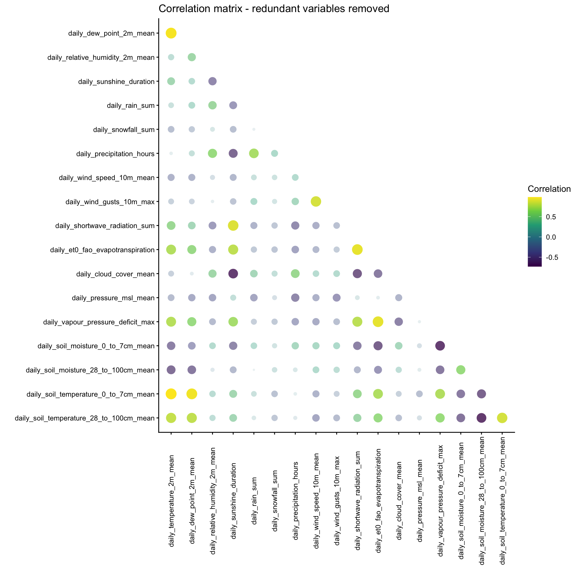
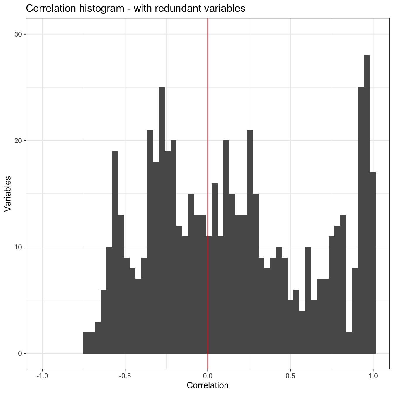
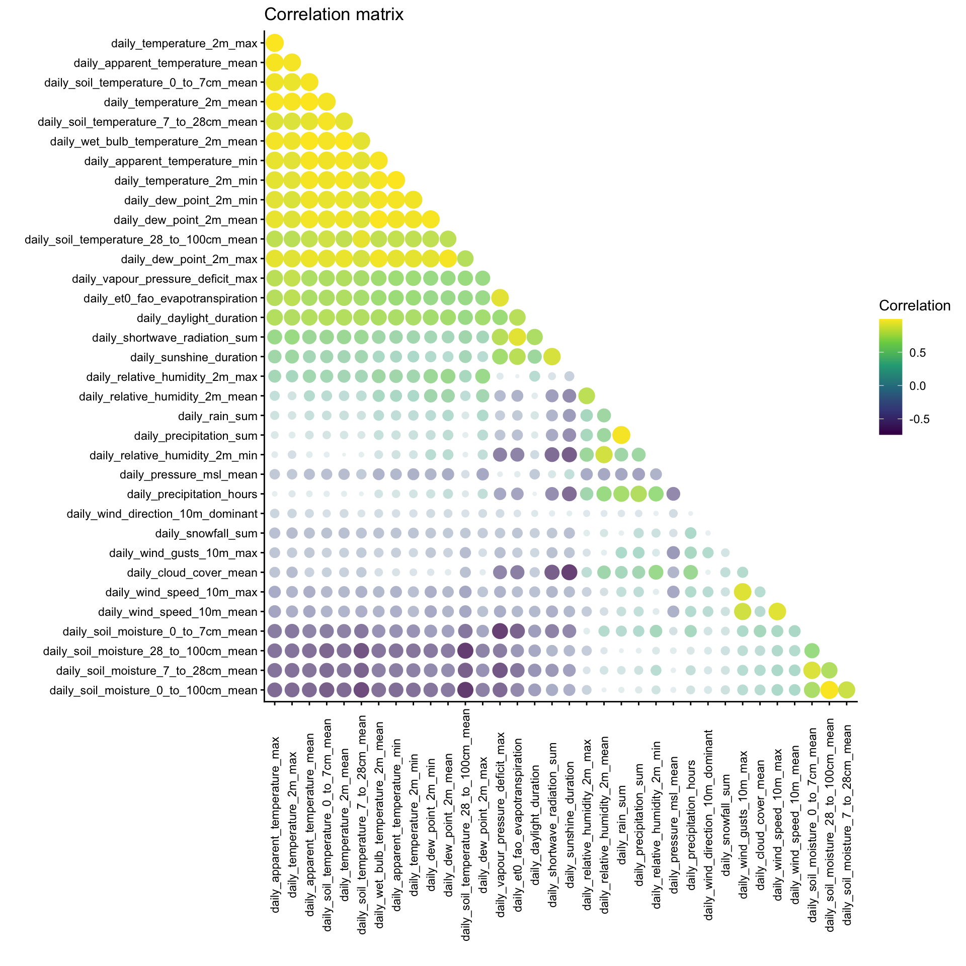
Some variables are highly correlated with other variables. While PCA will de-correlate the inputs and create orthogonal components, there will still be redundancy in the components because of the highly correlated input variables. In this code, I examine potentially redundant variables and remove them from the dataframe.

weather_vars <- weather_data |>
  select(
    daily_temperature_2m_mean:daily_soil_temperature_28_to_100cm_mean,
    -c(daily_sunrise, daily_sunset)
  )

weather_vars_cor <- weather_vars |>
  correlate() |>
  rearrange() |>
  shave()

cor_long <- weather_vars_cor |>
  pivot_longer(cols = -term) |>
  drop_na(value)

cor_long |>
  ggplot(aes(value)) +
  geom_histogram(bins = 50) +
  geom_vline(xintercept = 0, color = "red") +
  coord_cartesian(xlim = c(-1, 1), ylim = c(0, 30)) +
  labs(
    title = "Correlation histogram - with redundant variables",
    x = "Correlation",
    y = "Variables"
  )

cor_long |>
  summarize(mean_cor = mean(abs(value)), .by = term) |>
  arrange(term) |>
  print(n = Inf)

# A tibble: 34 × 2
   term                                    mean_cor
   <chr>                                      <dbl>
 1 daily_apparent_temperature_mean           0.980 
 2 daily_apparent_temperature_min            0.959 
 3 daily_cloud_cover_mean                    0.283 
 4 daily_daylight_duration                   0.738 
 5 daily_dew_point_2m_max                    0.929 
 6 daily_dew_point_2m_mean                   0.958 
 7 daily_dew_point_2m_min                    0.947 
 8 daily_et0_fao_evapotranspiration          0.709 
 9 daily_precipitation_hours                 0.274 
10 daily_precipitation_sum                   0.235 
11 daily_pressure_msl_mean                   0.255 
12 daily_rain_sum                            0.226 
13 daily_relative_humidity_2m_max            0.361 
14 daily_relative_humidity_2m_mean           0.323 
15 daily_relative_humidity_2m_min            0.276 
16 daily_shortwave_radiation_sum             0.558 
17 daily_snowfall_sum                        0.200 
18 daily_soil_moisture_0_to_100cm_mean       0.423 
19 daily_soil_moisture_0_to_7cm_mean         0.393 
20 daily_soil_moisture_28_to_100cm_mean      0.368 
21 daily_soil_moisture_7_to_28cm_mean        0.406 
22 daily_soil_temperature_0_to_7cm_mean      0.967 
23 daily_soil_temperature_28_to_100cm_mean   0.838 
24 daily_soil_temperature_7_to_28cm_mean     0.935 
25 daily_sunshine_duration                   0.454 
26 daily_temperature_2m_max                  0.994 
27 daily_temperature_2m_mean                 0.985 
28 daily_temperature_2m_min                  0.961 
29 daily_vapour_pressure_deficit_max         0.707 
30 daily_wet_bulb_temperature_2m_mean        0.970 
31 daily_wind_direction_10m_dominant         0.0891
32 daily_wind_gusts_10m_max                  0.207 
33 daily_wind_speed_10m_max                  0.288 
34 daily_wind_speed_10m_mean                 0.318 

rplot(weather_vars_cor) +
  scale_color_viridis_c() +
  labs(title = "Correlation matrix", color = "Correlation") +
  theme(axis.text.x = element_text(angle = 90, vjust = .5))

Here I select specific variables that are representative of the full set and rerun the correlation plots.

pca_inputs <- weather_data |>
  select(
    daily_temperature_2m_mean,
    daily_dew_point_2m_mean,
    daily_relative_humidity_2m_mean,
    daily_sunshine_duration,
    daily_rain_sum,
    daily_snowfall_sum,
    daily_precipitation_hours,
    daily_wind_speed_10m_mean,
    daily_wind_gusts_10m_max,
    daily_shortwave_radiation_sum,
    daily_et0_fao_evapotranspiration,
    daily_cloud_cover_mean,
    daily_relative_humidity_2m_mean,
    daily_pressure_msl_mean,
    daily_vapour_pressure_deficit_max,
    daily_soil_moisture_0_to_7cm_mean,
    daily_soil_moisture_28_to_100cm_mean,
    daily_soil_temperature_0_to_7cm_mean,
    daily_soil_temperature_28_to_100cm_mean
  ) |>
  select(where(is.numeric)) |>
  drop_bad_cols()

pca_inputs |>
  correlate() |>
  shave() |>
  rplot() +
  scale_color_viridis_c() +
  labs(
    title = "Correlation matrix - redundant variables removed",
    color = "Correlation"
  ) +
  theme(axis.text.x = element_text(angle = 90, vjust = .5))

pca_inputs |>
  correlate() |>
  rearrange() |>
  shave() |>
  pivot_longer(cols = -term) |>
  drop_na(value) |>
  ggplot(aes(value)) +
  geom_histogram(bins = 50) +
  geom_vline(xintercept = 0, color = "red") +
  coord_cartesian(xlim = c(-1, 1), ylim = c(0, 30)) +
  labs(
    title = "Correlation histogram - redundant variables removed",
    x = "Correlation",
    y = "Variables"
  )

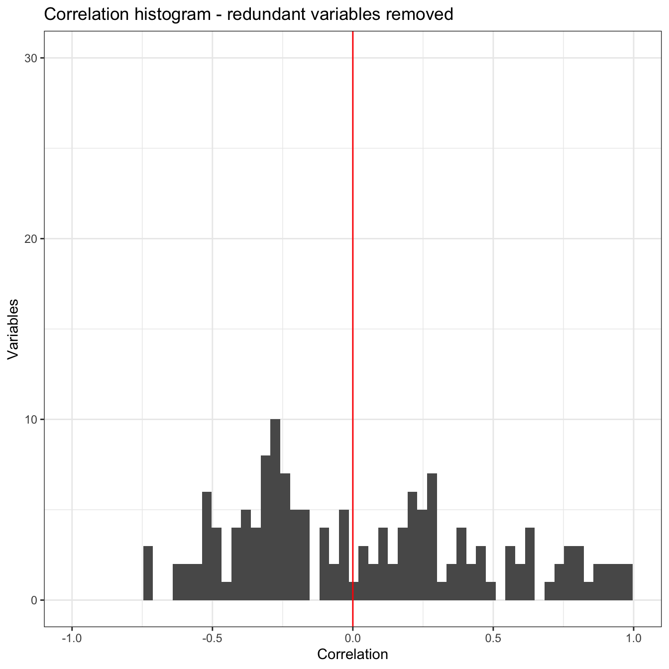
As expected, removing the redundant variables reduced the extent of correlation between the subsetted variables.

Principal component analysis (PCA)

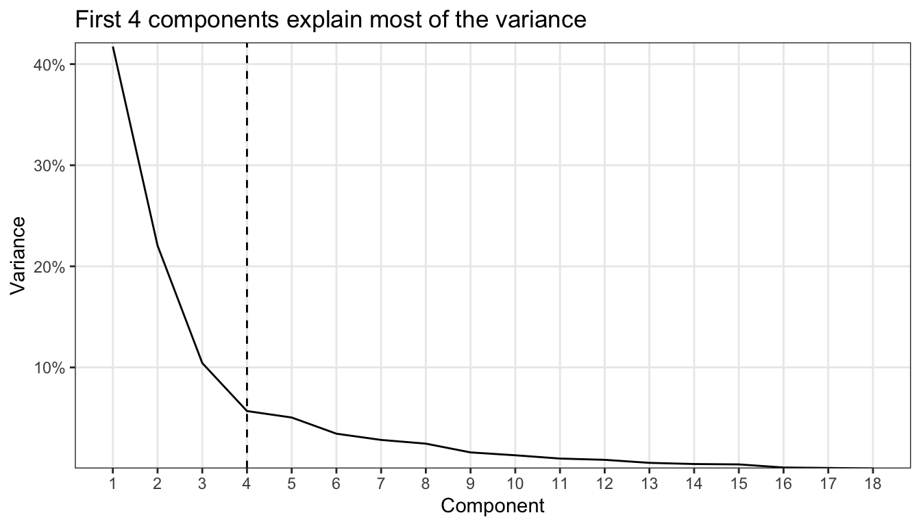
Next I fit PCA to the weather data. The first 4 components explain most of the variance, so I will focus on those.

pca_fit <- prcomp(pca_inputs, scale = TRUE)

pca_values <- pca_fit |>
  tidy(matrix = "eigenvalues")

pca_values |>
  ggplot(aes(PC, percent)) +
  geom_line() +
  geom_vline(xintercept = 4, lty = 2) +
  scale_x_continuous(breaks = 1:nrow(pca_values)) +
  scale_y_continuous(
    labels = percent_format(),
    expand = expansion(mult = c(0, 0.01))
  ) +
  labs(
    title = "First 4 components explain most of the variance",
    x = "Component",
    y = "Variance"
  ) +
  theme(panel.grid.minor = element_blank())

weather_data_pca <- pca_fit |>
  augment(weather_data) |>
  rename_with(~ str_replace(.x, "^.fittedPC", "pc")) |>
  select(all_of(names(weather_data_hist)), pc1:pc4)

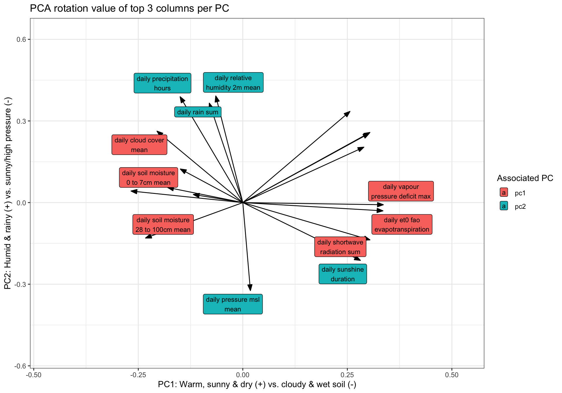
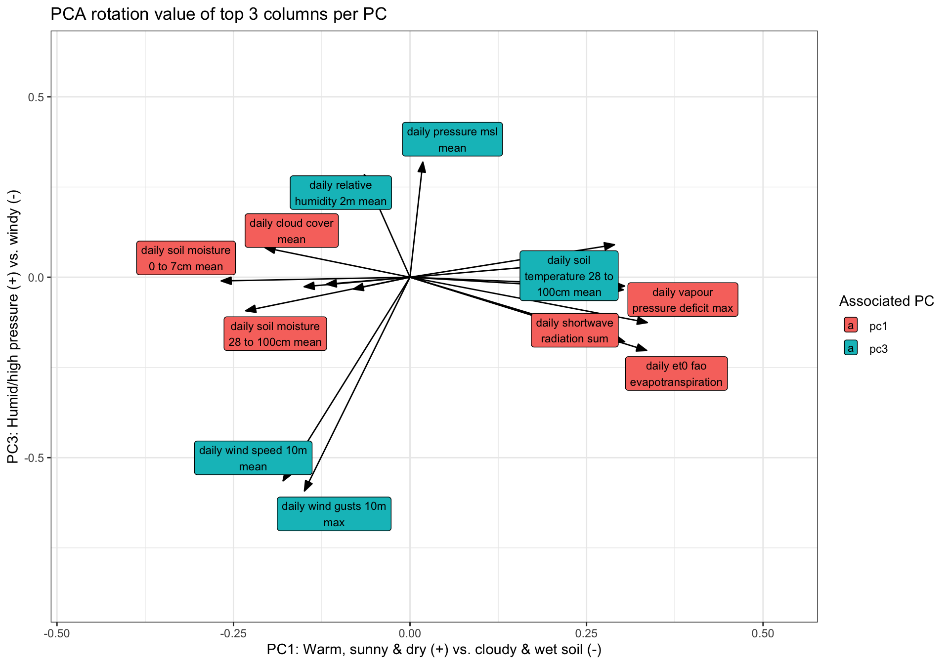
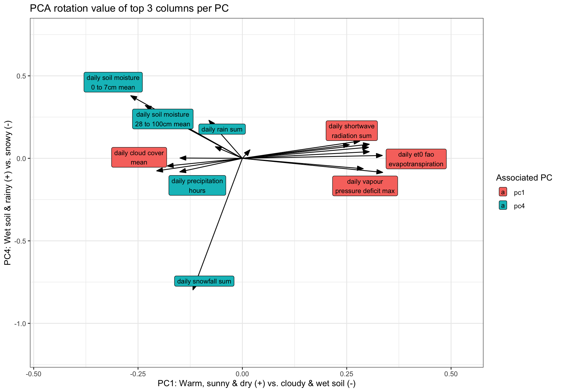
Next, I examine the variables that make up each component and assign labels that explain each component.

# define arrow style for plotting
arrow_style <- arrow(
  angle = 20,
  ends = "first",
  type = "closed",
  length = grid::unit(8, "pt")
)

# get rotation matrix
pca_rot <- pca_fit |>
  tidy(matrix = "rotation") |>
  pivot_wider(names_from = "PC", names_prefix = "PC", values_from = "value") |>
  rename_with(str_to_lower) |>
  select(column, pc1:pc4)

pca_rot_df_pos <- pca_rot |>
  pivot_longer(cols = -column, names_to = "pc", values_to = "pc_value") |>
  filter(pc_value > 0) |>
  group_by(pc) |>
  slice_max(order_by = pc_value, n = 3) |>
  ungroup()

pca_rot_df_neg <- pca_rot |>
  pivot_longer(cols = -column, names_to = "pc", values_to = "pc_value") |>
  filter(pc_value < 0) |>
  group_by(pc) |>
  slice_min(order_by = pc_value, n = 3) |>
  ungroup()

pca_rot_df <- bind_rows(pca_rot_df_pos, pca_rot_df_neg) |>
  select(pc, column, pc_value) |>
  arrange(pc, desc(pc_value))

print(pca_rot_df, n = Inf)

# A tibble: 24 × 3
   pc    column                                  pc_value
   <chr> <chr>                                      <dbl>
 1 pc1   daily_vapour_pressure_deficit_max         0.336 
 2 pc1   daily_et0_fao_evapotranspiration          0.335 
 3 pc1   daily_shortwave_radiation_sum             0.304 
 4 pc1   daily_cloud_cover_mean                   -0.205 
 5 pc1   daily_soil_moisture_28_to_100cm_mean     -0.233 
 6 pc1   daily_soil_moisture_0_to_7cm_mean        -0.267 
 7 pc2   daily_relative_humidity_2m_mean           0.392 
 8 pc2   daily_precipitation_hours                 0.389 
 9 pc2   daily_rain_sum                            0.366 
10 pc2   daily_shortwave_radiation_sum            -0.137 
11 pc2   daily_sunshine_duration                  -0.212 
12 pc2   daily_pressure_msl_mean                  -0.323 
13 pc3   daily_pressure_msl_mean                   0.319 
14 pc3   daily_relative_humidity_2m_mean           0.284 
15 pc3   daily_soil_temperature_28_to_100cm_mean   0.0901
16 pc3   daily_et0_fao_evapotranspiration         -0.203 
17 pc3   daily_wind_speed_10m_mean                -0.564 
18 pc3   daily_wind_gusts_10m_max                 -0.592 
19 pc4   daily_soil_moisture_0_to_7cm_mean         0.380 
20 pc4   daily_soil_moisture_28_to_100cm_mean      0.321 
21 pc4   daily_rain_sum                            0.231 
22 pc4   daily_precipitation_hours                -0.0818
23 pc4   daily_vapour_pressure_deficit_max        -0.0852
24 pc4   daily_snowfall_sum                       -0.797 

pc_labels <- list(
  pc1 = "PC1: Warm, sunny & dry (+) vs. cloudy & wet soil (-)",
  pc2 = "PC2: Humid & rainy (+) vs. sunny/high pressure (-)",
  pc3 = "PC3: Humid/high pressure (+) vs. windy (-)",
  pc4 = "PC4: Wet soil & rainy (+) vs. snowy (-)"
)

pc_labels_df <- enframe(pc_labels, name = "pc", value = "pc_label") |>
  mutate(pc_label = map_chr(pc_label, 1)) |>
  mutate(pc_label = str_wrap(pc_label, 40))

pc_label <- function(x) {
  pluck(pc_labels, x)
}

These scatter plots show the rotation values of the weather variables that are most integral to each principal component.

graph_pca_rot <- function(pca_df, x, y) {
  pca_points_x <- pca_rot_df |>
    filter(pc == x)

  pca_points_x <- pca_points_x |>
    inner_join(pca_df, pca_points_x, by = "column") |>
    mutate(text = str_replace_all(column, "_", " ") |> str_wrap(20))

  pca_points_y <- pca_rot_df |>
    filter(pc == y)

  pca_points_y <- pca_points_y |>
    inner_join(pca_df, pca_points_y, by = "column") |>
    mutate(text = str_replace_all(column, "_", " ") |> str_wrap(20))

  pca_points <- bind_rows(pca_points_x, pca_points_y) |>
    group_by(column) |>
    filter(abs(pc_value) == max(abs(pc_value))) |>
    ungroup()

  pca_df <- pca_df |>
    select(column, all_of(c(x, y)))

  pca_df |>
    mutate(text = str_replace_all(column, "_", " ") |> str_wrap(20)) |>
    ggplot(aes(.data[[x]], .data[[y]])) +
    geom_segment(xend = 0, yend = 0, arrow = arrow_style) +
    geom_label_repel(
      data = pca_points,
      aes(label = text, fill = pc),
      size = 3
    ) +
    scale_x_continuous(expand = expansion(mult = .4)) +
    scale_y_continuous(expand = expansion(mult = .4)) +
    labs(
      title = "PCA rotation value of top 3 columns per PC",
      x = pc_label(x),
      y = pc_label(y),
      fill = "Associated PC"
    )
}

pca_rot |>
  graph_pca_rot("pc1", "pc2")

pca_rot |>
  graph_pca_rot("pc1", "pc3")

pca_rot |>
  graph_pca_rot("pc1", "pc4")

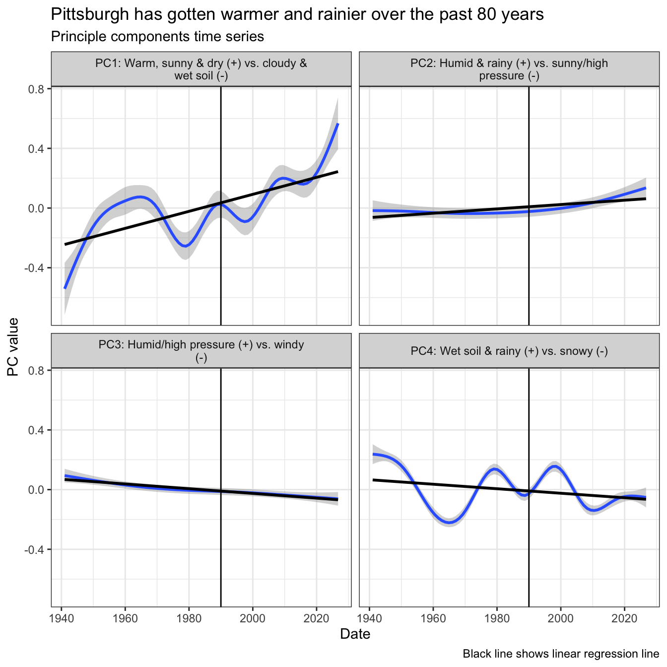
Next I graph the principal components over time. PCs 1, 2, and 3 have clearly changed over time. PC 4 is very noisy, but also decreased.

weather_data_pca |>
  select(date, pc1:pc4) |>
  pivot_longer(cols = starts_with("pc"), names_to = "pc") |>
  left_join(pc_labels_df) |>
  ggplot(aes(date, value)) +
  geom_smooth() +
  geom_smooth(method = "lm", color = "black", se = FALSE) +
  geom_vline(xintercept = str_c(year_cutoff, "-01-01") |> ymd()) +
  facet_wrap(vars(str_wrap(pc_label, 40))) +
  labs(
    title = "Pittsburgh has gotten warmer and rainier over the past 80 years",
    subtitle = "Principle components time series",
    x = "Date",
    y = "PC value",
    caption = "Black line shows linear regression line"
  )

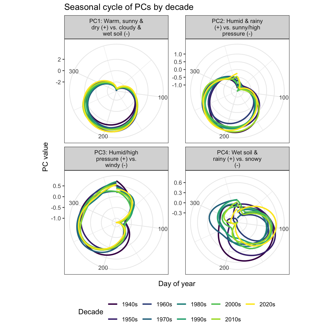
This polar chart shows the cyclicality of the components by decade. The circular axis is the day of the year (starting at day 1), and the axis going away from the center is the value of the principle component.

weather_pca_long <- weather_data_pca |>
  select(yday, year, decade, pc1:pc4) |>
  pivot_longer(cols = starts_with("pc"), names_to = "pc") |>
  left_join(pc_labels_df, by = "pc")

weather_pca_long |>
  ggplot(aes(yday, value, color = decade)) +
  geom_smooth(se = FALSE) +
  scale_color_viridis_d() +
  coord_polar() +
  facet_wrap(vars(str_wrap(pc_label, 20)), scales = "free_y") +
  labs(
    title = "Seasonal cycle of PCs by decade",
    x = "Day of year",
    y = "PC value",
    color = "Decade"
  ) +
  theme(legend.position = "bottom", legend.direction = "horizontal")

Component 4 has changed the most across the time series. The soil held much more moisture in the early decades.

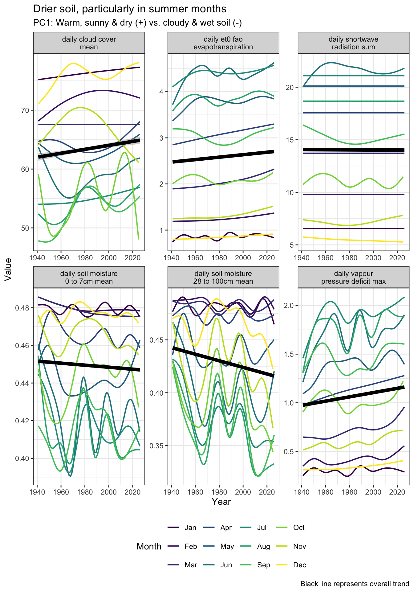
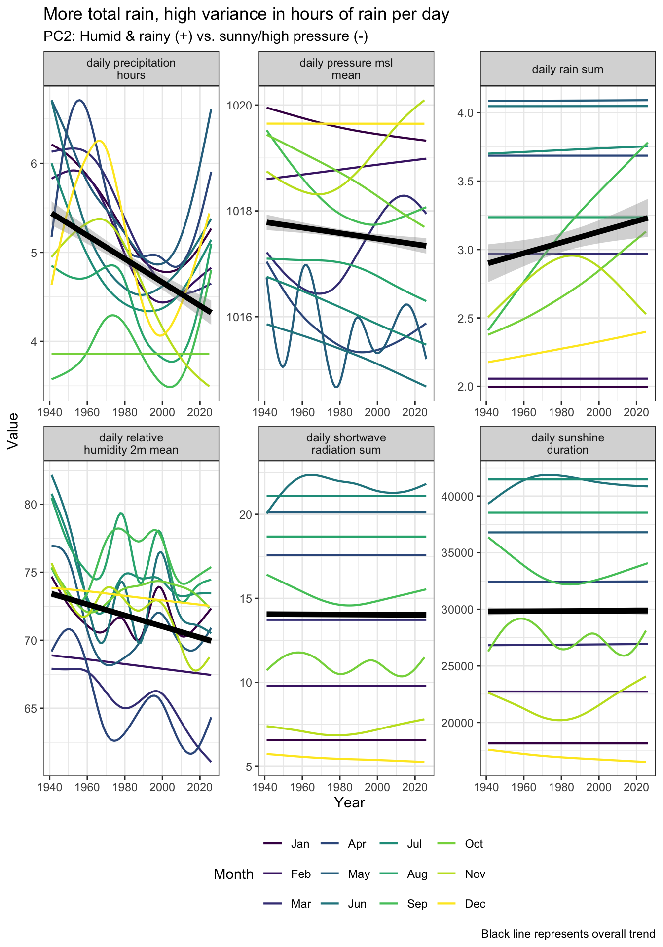
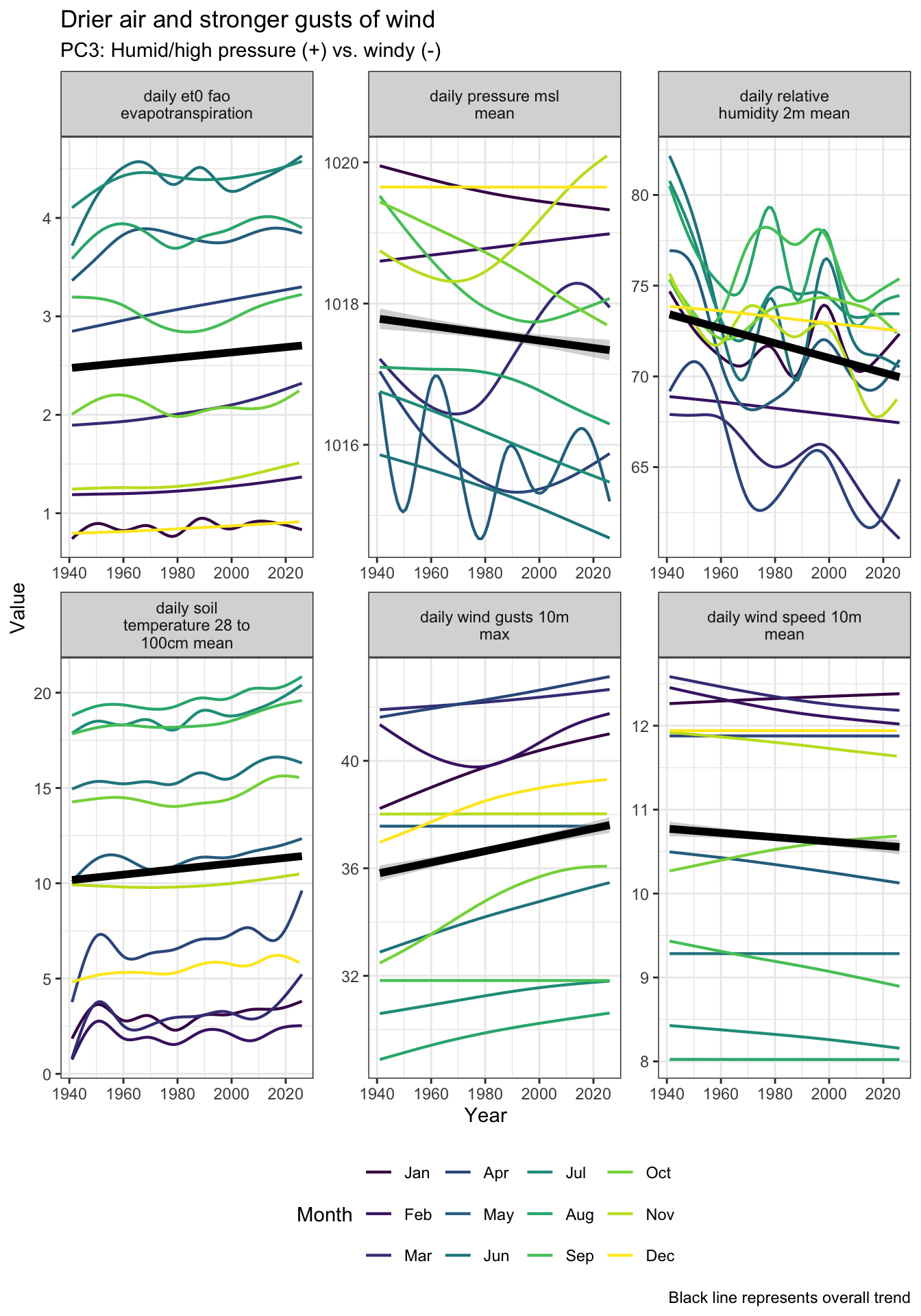
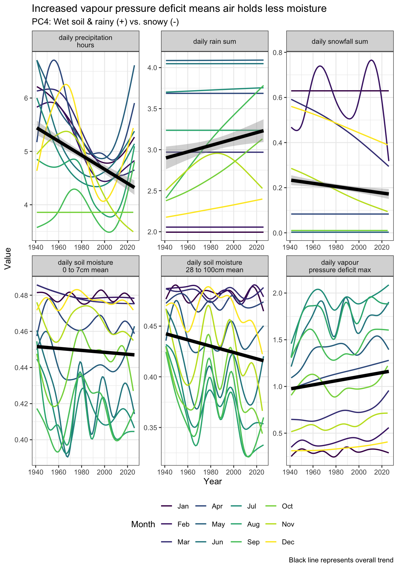
Next, I plot the time series of the weather variables for each component, broken out by month.

pc_column_line_plot <- function(x, title_text = "") {
  pc_cols <- pca_rot_df |>
    filter(pc == x) |>
    pull(column)

  weather_data_pca |>
    select(year, month, all_of(pc_cols)) |>
    pivot_longer(cols = all_of(pc_cols)) |>
    mutate(name = str_replace_all(name, "_", " ") |> str_wrap(20)) |>
    ggplot(aes(x = year, y = value)) +
    geom_smooth(aes(color = month, group = month), se = FALSE, lwd = .75) +
    geom_smooth(method = "lm", color = "black", lwd = 2) +
    facet_wrap(vars(name), scales = "free") +
    labs(
      title = title_text,
      subtitle = pc_label(x),
      caption = "Black line represents overall trend",
      x = "Year",
      y = "Value",
      color = "Month"
    ) +
    theme(legend.position = "bottom", legend.direction = "horizontal")
}

pc_column_line_plot(
  "pc1",
  title_text = "Drier soil, particularly in summer months"
)

pc_column_line_plot(
  "pc2",
  title_text = "More total rain, high variance in hours of rain per day"
)

pc_column_line_plot("pc3", title_text = "Drier air and stronger gusts of wind")

pc_column_line_plot(
  "pc4",
  title_text = "Increased vapour pressure deficit means air holds less moisture"
)

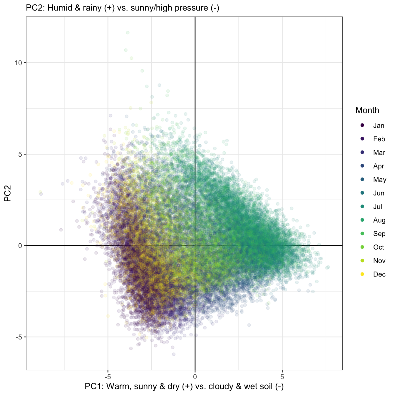
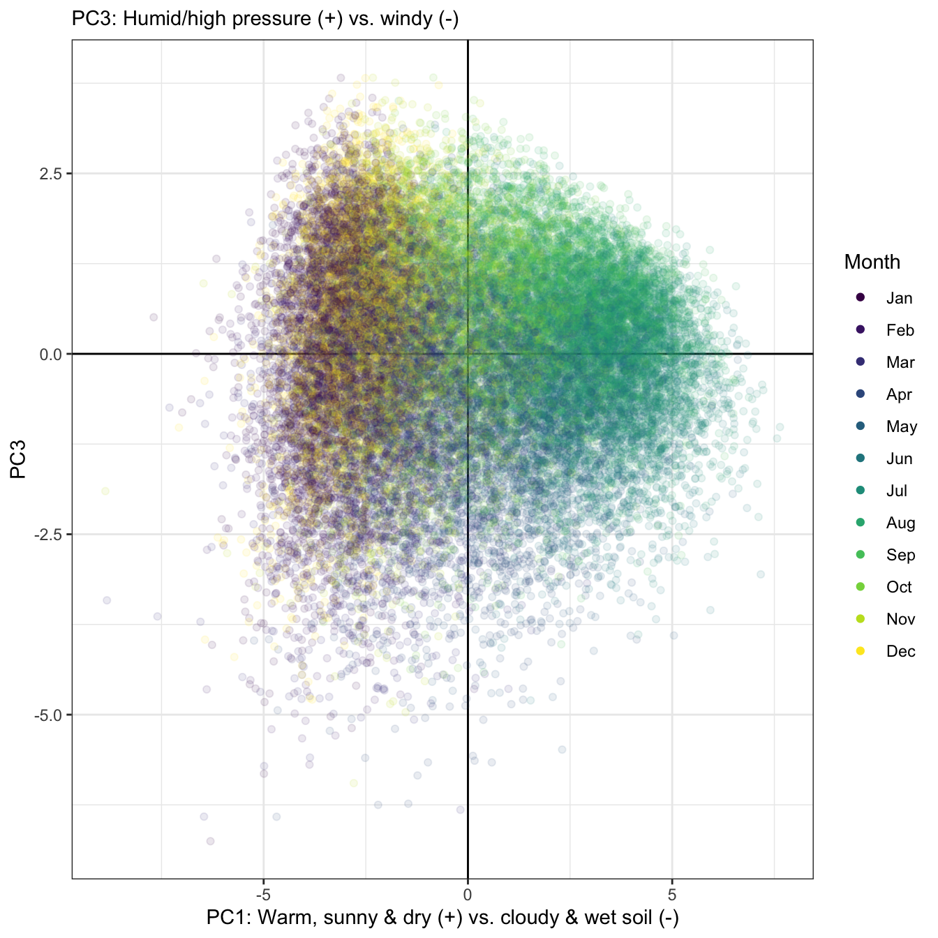
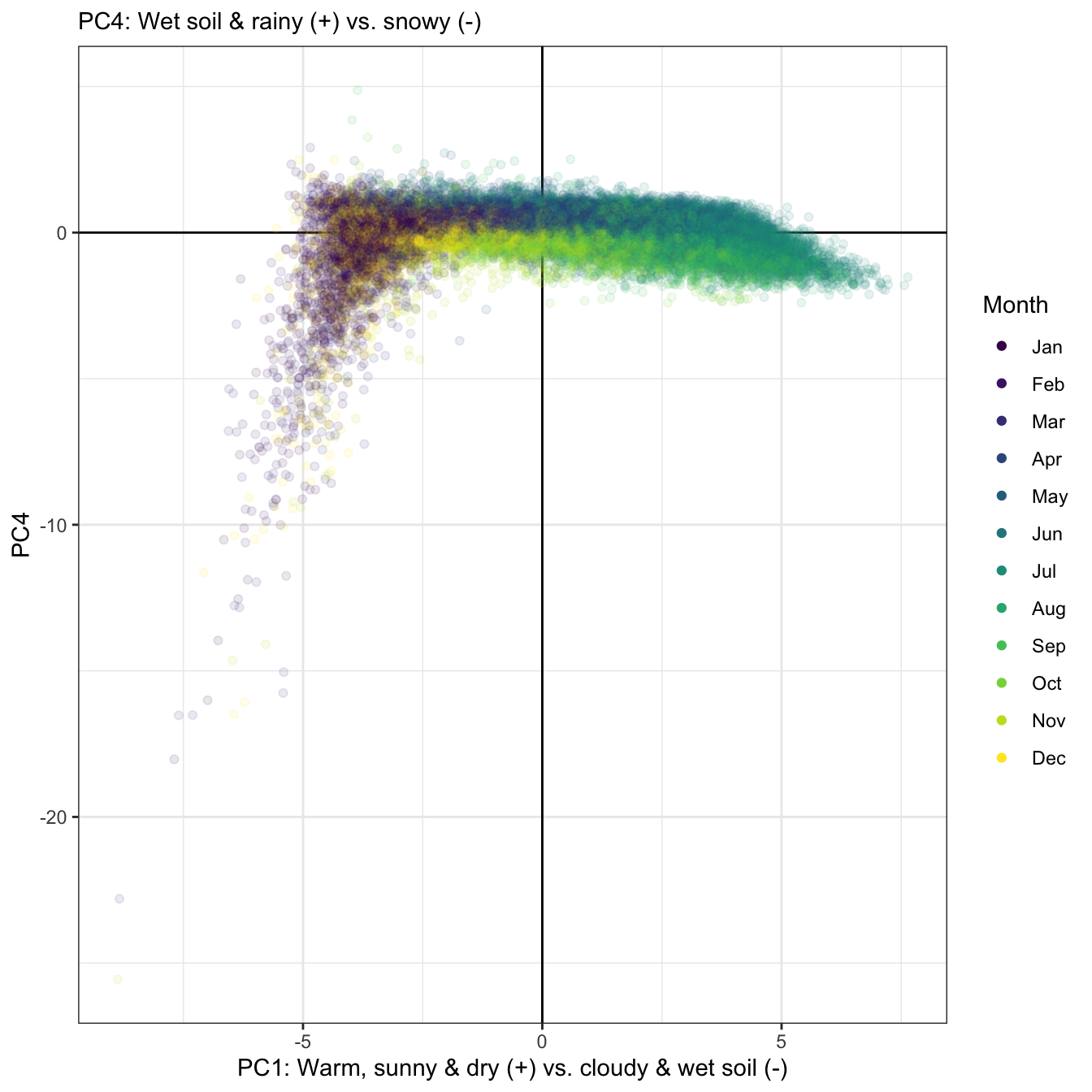
These scatter plots show the first component vs. principal components 2-4. There are not distinct non-overlapping groupings, and the months represent gradients of a continuous signal, not discrete categories. This shows that weather in Pittsburgh is highly variable and is not easily representable by distinct clusters.

pca_scatter <- function(pca_df, x, y, color_var) {
  pca_df |>
    ggplot(aes(.data[[x]], .data[[y]], color = .data[[color_var]])) +
    geom_vline(xintercept = 0) +
    geom_hline(yintercept = 0) +
    geom_point(size = 1.5, alpha = .1) +
    guides(color = guide_legend(override.aes = list(alpha = 1))) +
    labs(
      x = pc_label(x) |> str_wrap(70),
      y = str_to_upper(y),
      subtitle = pc_label(y) |> str_wrap(70),
      color = "Month"
    )
}

pca_scatter(weather_data_pca, "pc1", "pc2", "month")

pca_scatter(weather_data_pca, "pc1", "pc3", "month")

pca_scatter(weather_data_pca, "pc1", "pc4", "month")

The sharp non-linear curve downward along PC4 shows that very snowy days are very distinct compared to other weather patterns.

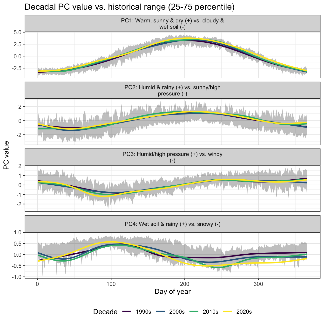
Finally, I plot the recent values of the components by decade, with the historical range annotated in grey.

weather_data_hist_pca <- weather_data_pca |>
  filter(year < year_cutoff) |>
  select(date, month, decade, yday, year, starts_with("pc"))

weather_data_recent_pca <- weather_data_pca |>
  filter(year >= year_cutoff) |>
  select(date, month, decade, yday, year, starts_with("pc"))

quantile_df <- function(x, probs = c(0.25, 0.5, 0.75)) {
  tibble(
    val = quantile(x, probs, na.rm = TRUE),
    quant = probs
  )
}

historical_range <- weather_data_hist_pca |>
  select(date, yday, pc1:pc4) |>
  pivot_longer(cols = starts_with("pc"), names_to = "pc") |>
  reframe(quantile_df(value), .by = c(yday, pc)) |>
  pivot_wider(names_from = quant, values_from = val, names_prefix = "pct_") |>
  arrange(pc, yday) |>
  left_join(pc_labels_df, by = "pc")

weather_pca_recent_long <- weather_data_recent_pca |>
  select(yday, year, decade, pc1:pc4) |>
  pivot_longer(cols = starts_with("pc"), names_to = "pc") |>
  left_join(pc_labels_df, by = "pc")

weather_pca_recent_long |>
  ggplot(aes(yday, value, group = year)) +
  geom_ribbon(
    data = historical_range,
    aes(x = yday, ymin = pct_0.25, ymax = pct_0.75),
    alpha = .3,
    inherit.aes = FALSE
  ) +
  geom_smooth(aes(group = decade, color = decade), lwd = 1, se = FALSE) +
  facet_wrap(vars(pc_label), ncol = 1, scales = "free_y") +
  scale_color_viridis_d() +
  labs(
    title = "Decadal PC value vs. historical range (25-75 percentile)",
    x = "Day of year",
    y = "PC value",
    color = "Decade"
  ) +
  theme(legend.position = "bottom", legend.direction = "horizontal")

In the 2020s, the soil moisture in fall and winter has fallen below the historical range.