Model discussion

I trained 3 models against the assessment data:

Linear model
Random Forest
Bagged Tree

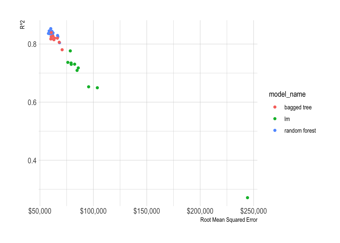
I chose the Bagged Tree model because it performed about as well as the Random Forest model, but it predicts against new data much faster. Prediction speed is important because the UI for the dashboard has to update very quickly.

Total observations: 120,872

Training set metrics (75% of total observations)

I used 10-fold cross-validation to assess model performance against the training set:

train_metrics %>% 
  select(model_name, id, .metric, .estimate) %>% 
  pivot_wider(names_from = .metric, values_from = .estimate) %>% 
  ggplot(aes(rmse, rsq, color = model_name)) +
  geom_point() +
  scale_x_continuous(label = dollar) +
  labs(x = "Root Mean Squared Error",
       y = "R^2")

Test set metrics (25% of total observations)

test_metrics %>% 
  select(.metric, .estimate)

# A tibble: 3 × 2
  .metric   .estimate
  <chr>         <dbl>
1 rmse     251406.   
2 rsq           0.607
3 mape    3724488.

model_results %>% 
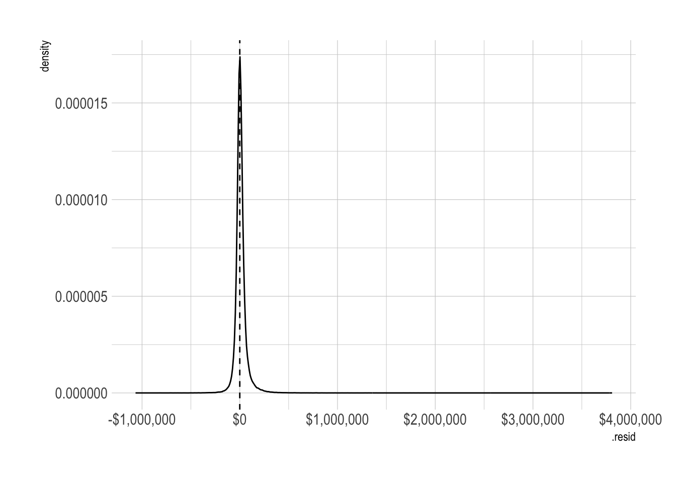
  ggplot(aes(.resid)) +
  geom_density() +
  geom_vline(xintercept = 0, lty = 2) +
  scale_x_continuous(label = label_dollar())

model_results %>% 
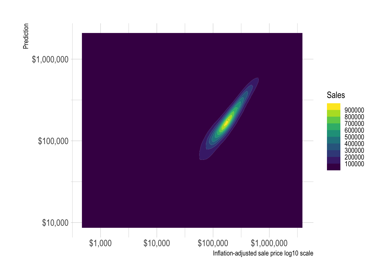
  ggplot(aes(sale_price_adj, .pred_dollar)) +
  geom_density_2d_filled(contour_var = "count") +
  scale_x_log10(label = label_dollar()) +
  scale_y_log10(label = label_dollar()) +
  guides(fill = guide_coloursteps()) +
  labs(x = "Inflation-adjusted sale price log10 scale",
       y = "Prediction",
       fill = "Sales")

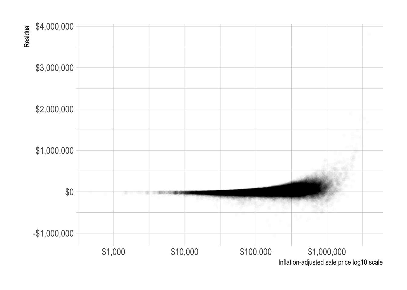
The model becomes less effective as the actual sale price increases.

model_results %>% 
  ggplot(aes(sale_price_adj, .resid)) +
  geom_point(alpha = .01) +
  scale_x_log10(label = dollar) +
  scale_y_continuous(label = dollar) +
  labs(x = "Inflation-adjusted sale price log10 scale",
       y = "Residual")

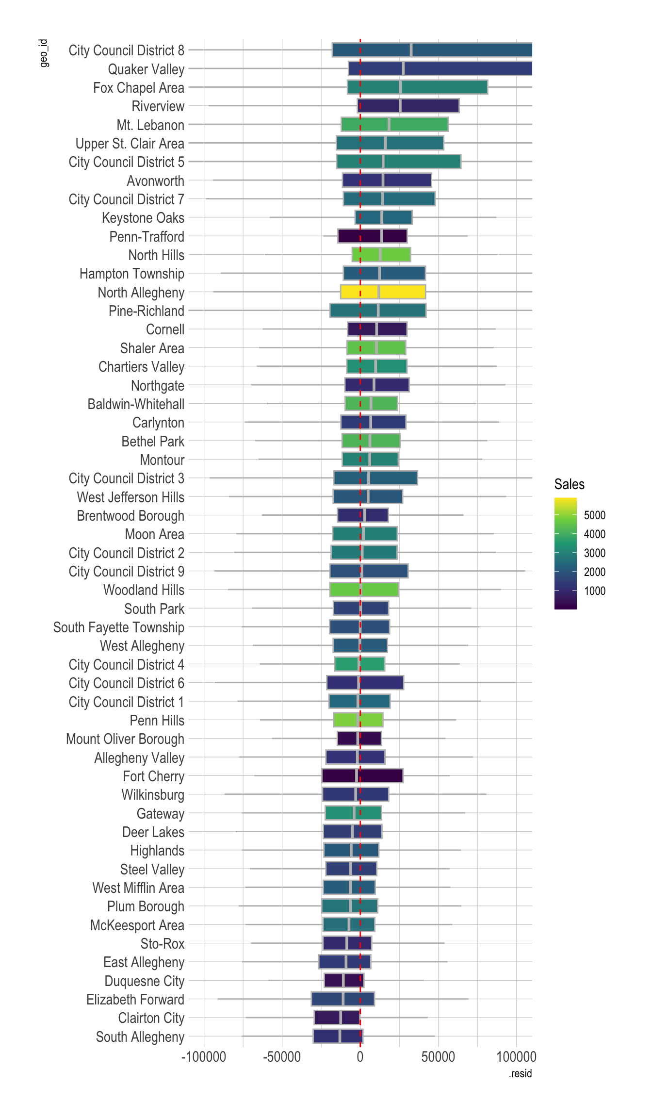
geo_ids <- st_read("post_data/unified_geo_ids/unified_geo_ids.shp",
                   quiet = T)

geo_id_median_resid <- model_results %>% 
  group_by(geo_id) %>% 
  summarize(median_resid = median(.resid))

pal <- colorNumeric(
  palette = "viridis",
  domain = geo_id_median_resid$median_resid)

geo_ids %>% 
  left_join(geo_id_median_resid) %>% 
  leaflet() %>% 
  addProviderTiles(providers$OpenStreetMap.Mapnik,
                   options = providerTileOptions(noWrap = TRUE,
                                                 minZoom = 9
                                                 #maxZoom = 8
                   )) %>%
  addPolygons(popup = ~ str_c(geo_id, " ", "median residual: ", round(median_resid, 2), sep = ""),
              fillColor = ~pal(median_resid),
              fillOpacity = .7,
              color = "black",
              weight = 3) %>% 
  addLegend("bottomright", pal = pal, values = ~median_resid,
            title = "Median of residual",
            opacity = 1)

Joining with `by = join_by(geo_id)`

model_results %>% 
  add_count(geo_id) %>% 
  mutate(geo_id = fct_reorder(geo_id, .resid, .fun = median)) %>% 
  ggplot(aes(.resid, geo_id, fill = n)) +
  geom_boxplot(color = "grey",
               outlier.alpha = 0) +
  geom_vline(xintercept = 0, lty = 2, color = "red") +
  scale_fill_viridis_c() +
  coord_cartesian(xlim = c(-10^5, 10^5)) +
  labs(fill = "Sales")

model_results %>% 
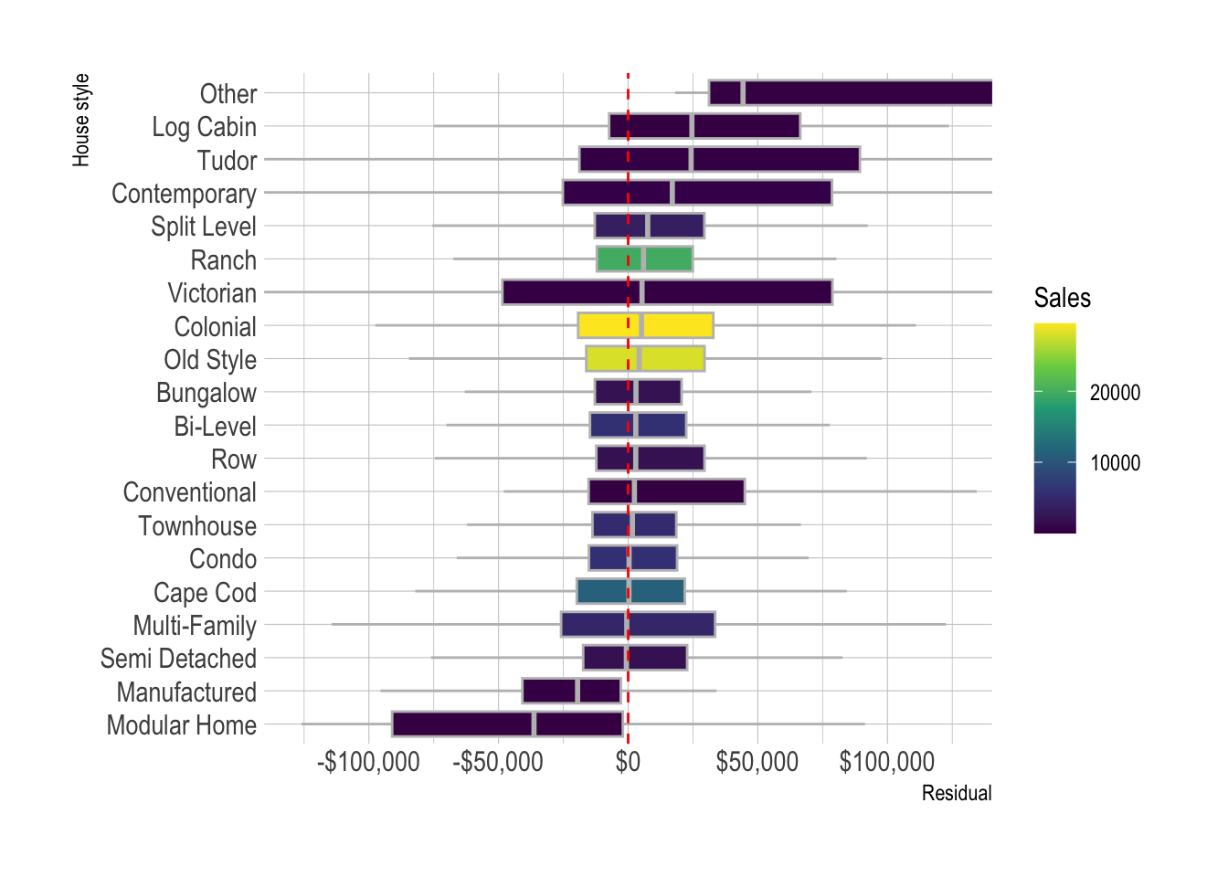
  add_count(style_desc) %>% 
  mutate(style_desc = fct_reorder(style_desc, .resid, .fun = median)) %>% 
  ggplot(aes(.resid, style_desc, fill = n)) +
  geom_boxplot(color = "grey",
               outlier.alpha = 0) +
  geom_vline(xintercept = 0, lty = 2, color = "red") +
  coord_cartesian(xlim = c(-10.5^5, 10.5^5)) +
  scale_x_continuous(labels = label_dollar()) +
  scale_fill_viridis_c() +
  labs(fill = "Sales",
       x = "Residual",
       y = "House style")

model_results %>% 
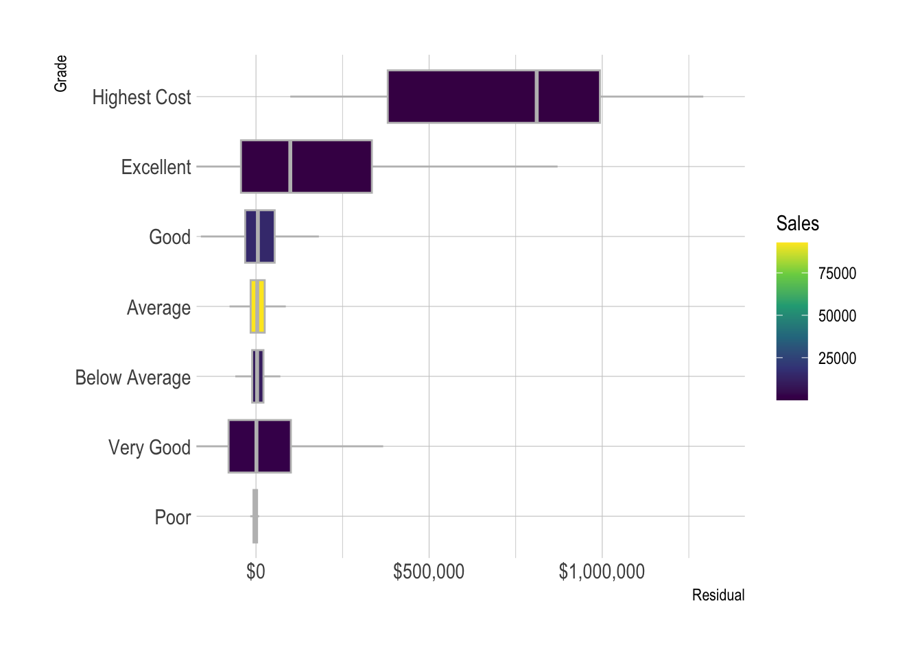
  add_count(grade_desc) %>% 
  mutate(grade_desc = fct_reorder(grade_desc, .resid, .fun = median)) %>% 
  ggplot(aes(.resid, grade_desc, fill = n)) +
  geom_boxplot(color = "grey",
               outlier.alpha = 0) +
  scale_fill_viridis_c() +
  scale_x_continuous(labels = label_dollar()) +
  coord_cartesian(xlim = c(-10^5, 10.5^6)) +
  labs(x = "Residual",
       y = "Grade",
       fill = "Sales")

model_results %>% 
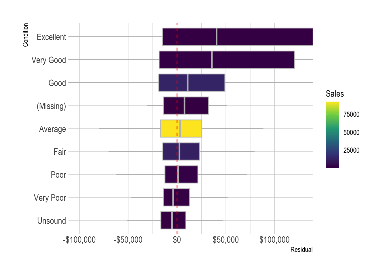
  add_count(condition_desc) %>% 
  mutate(condition_desc = fct_explicit_na(condition_desc),
         condition_desc = fct_reorder(condition_desc, .resid, .fun = median)) %>% 
  ggplot(aes(.resid, condition_desc, fill = n)) +
  geom_boxplot(color = "grey",
               outlier.alpha = 0) +
  geom_vline(xintercept = 0, lty = 2, color = "red") +
  scale_fill_viridis_c() +
  scale_x_continuous(labels = label_dollar()) +
  coord_cartesian(xlim = c(-10^5, 10.5^5)) +
  labs(x = "Residual",
       y = "Condition",
       fill = "Sales")

Warning: There was 1 warning in `mutate()`.
ℹ In argument: `condition_desc = fct_explicit_na(condition_desc)`.
Caused by warning:
! `fct_explicit_na()` was deprecated in forcats 1.0.0.
ℹ Please use `fct_na_value_to_level()` instead.

model_results %>% 
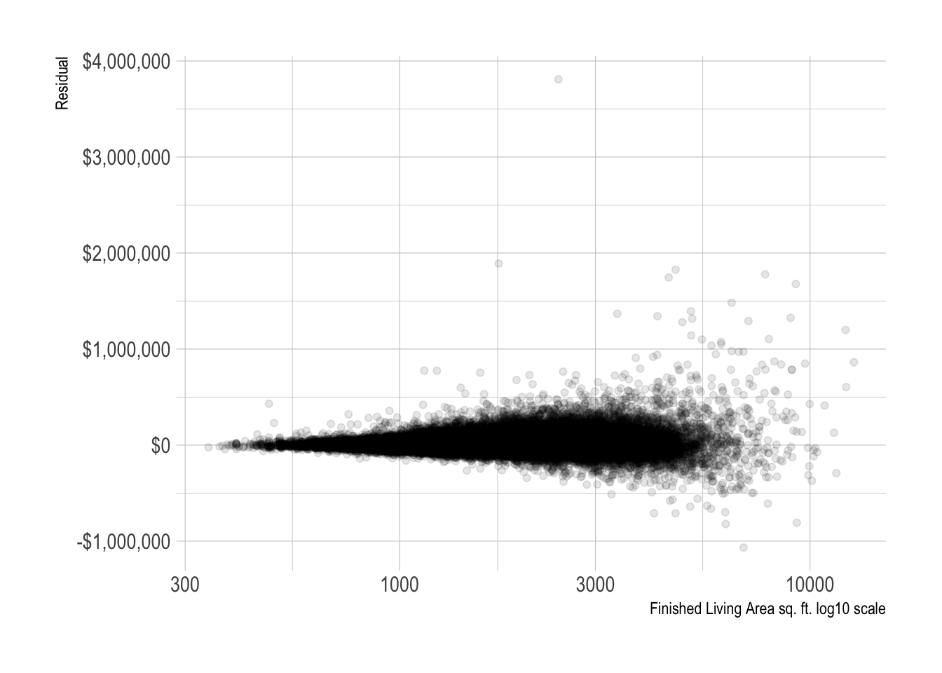
  ggplot(aes(finished_living_area, .resid)) +
  geom_point(alpha = .1) +
  scale_x_log10() +
  scale_y_continuous(label = dollar) +
  labs(x = "Finished Living Area sq. ft. log10 scale",
       y = "Residual")

model_results %>% 
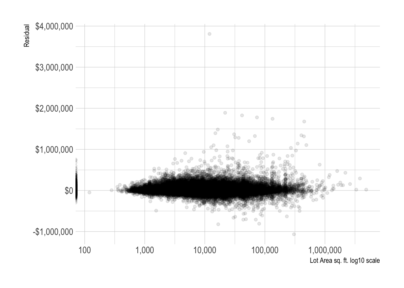
  ggplot(aes(lot_area, .resid)) +
  geom_point(alpha = .1) +
  scale_x_log10(labels = label_comma()) +
  scale_y_continuous(labels = label_dollar()) +
  labs(x = "Lot Area sq. ft. log10 scale",
       y = "Residual")

Warning: Transformation introduced infinite values in continuous x-axis

model_results %>% 
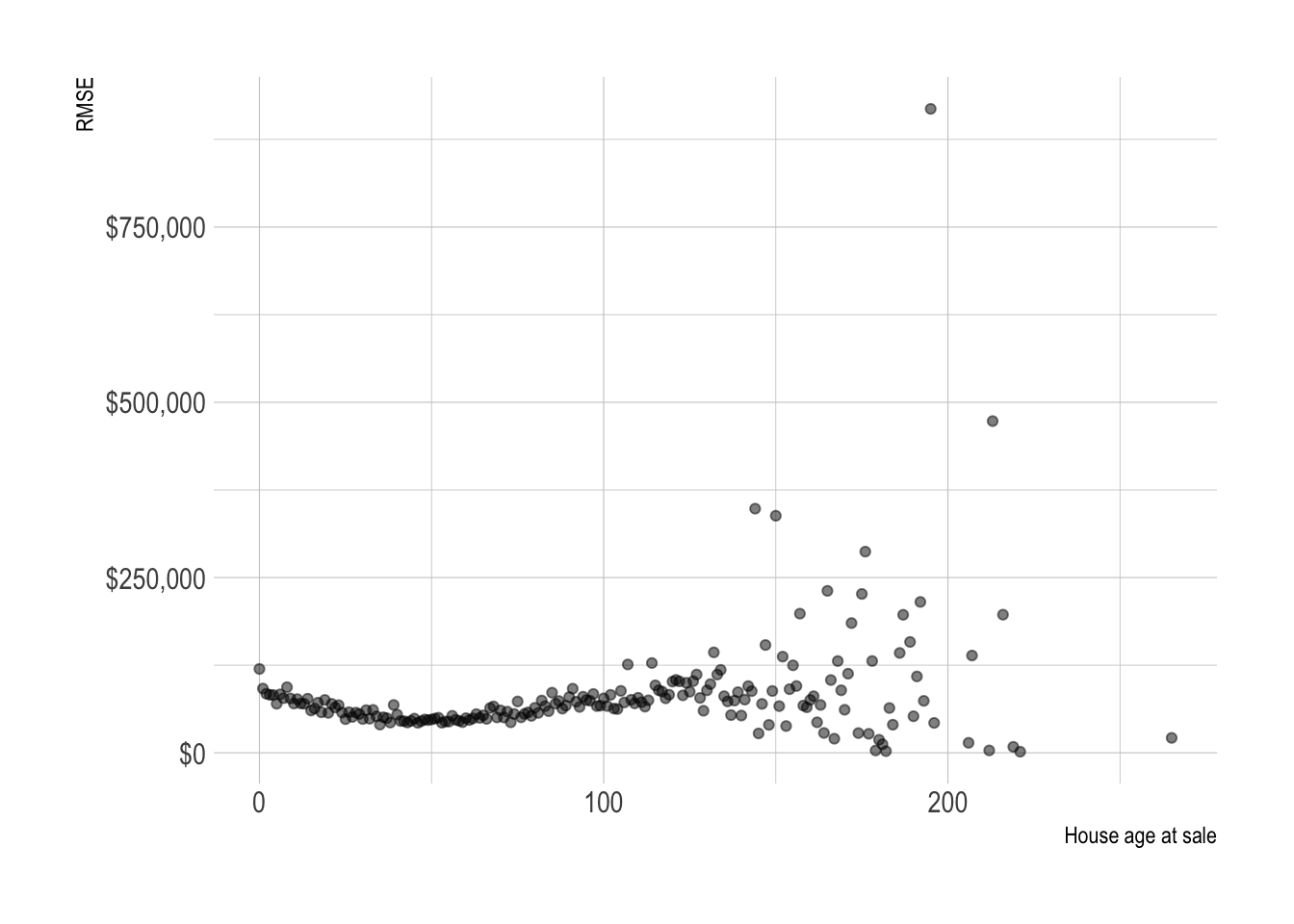
  group_by(house_age_at_sale) %>% 
  rmse(truth = sale_price_adj, estimate = .pred_dollar) %>% 
  ggplot(aes(house_age_at_sale, .estimate)) +
  geom_point(alpha = .5) +
  scale_y_continuous(labels = label_dollar()) +
  labs(x = "House age at sale",
       y = "RMSE")

The model is best at predicting the sale price of houses built in the 1940s to 1980s. This is when most of the houses in the county were built.

model_results %>% 
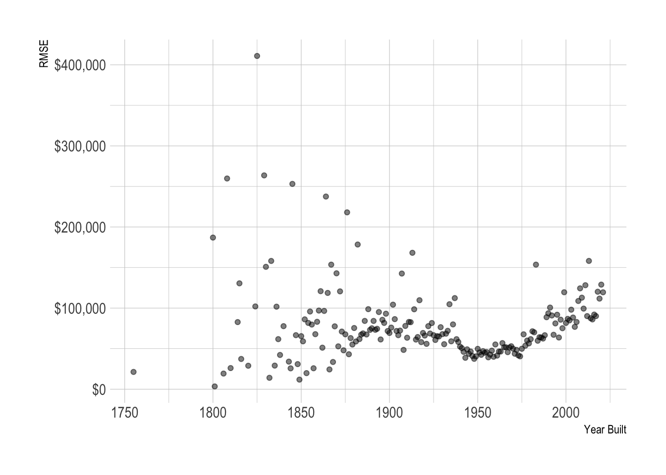
  group_by(year_built) %>% 
  rmse(truth = sale_price_adj, estimate = .pred_dollar) %>% 
  ggplot(aes(year_built, .estimate)) +
  geom_point(alpha = .5) +
  scale_y_continuous(labels = label_dollar()) +
  labs(x = "Year Built",
       y = "RMSE")

model_results %>% 
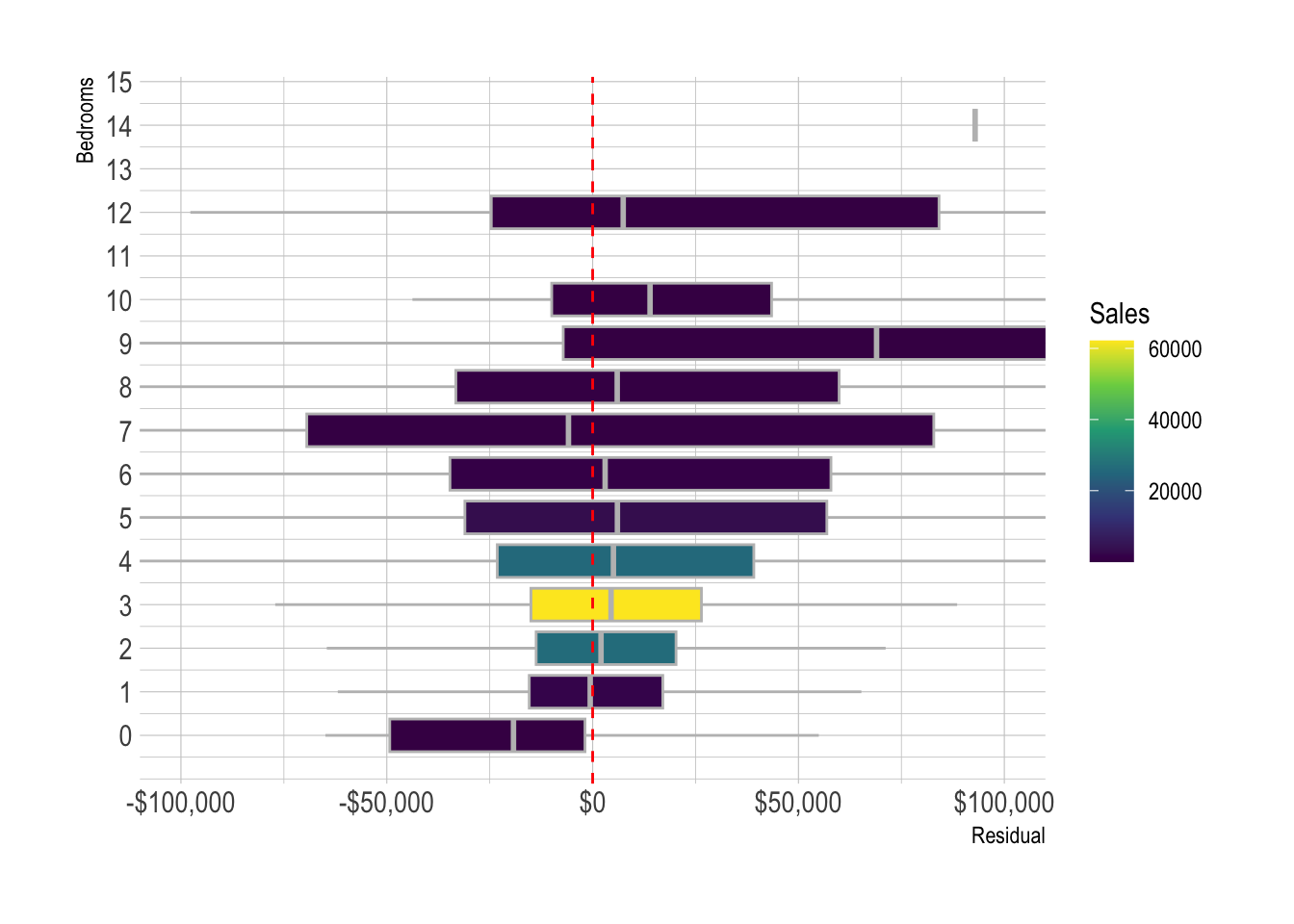
  add_count(bedrooms) %>% 
  ggplot(aes(.resid, bedrooms, group = bedrooms, fill = n)) +
  geom_boxplot(color = "grey",
               outlier.alpha = 0) +
  geom_vline(xintercept = 0, lty = 2, color = "red") +
  scale_y_continuous(breaks = c(0:15)) +
  scale_fill_viridis_c() +
  scale_x_continuous(labels = label_dollar()) +
  coord_cartesian(xlim = c(-10^5, 10^5)) +
  labs(x = "Residual",
       y = "Bedrooms",
       fill = "Sales")

Warning: Removed 2 rows containing missing values (`stat_boxplot()`).

model_results %>% 
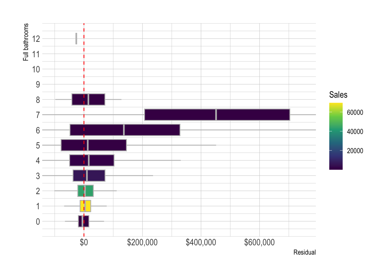
  add_count(full_baths) %>% 
  ggplot(aes(.resid, full_baths, group = full_baths, fill = n)) +
  geom_boxplot(color = "grey",
               outlier.alpha = 0) +
  geom_vline(xintercept = 0, lty = 2, color = "red") +
  scale_y_continuous(breaks = c(0:12)) +
  scale_fill_viridis_c() +
  scale_x_continuous(label = dollar) +
  coord_cartesian(xlim = c(-10^5, 750000)) +
  labs(x = "Residual",
       y = "Full bathrooms",
       fill = "Sales")

Warning: Removed 14 rows containing missing values (`stat_boxplot()`).

model_results %>% 
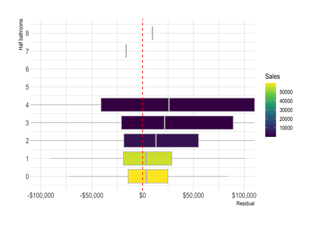
  add_count(half_baths) %>% 
  ggplot(aes(.resid, half_baths, group = half_baths, fill = n)) +
  geom_boxplot(color = "grey",
               outlier.alpha = 0) +
  geom_vline(xintercept = 0, lty = 2, color = "red") +
  scale_y_continuous(breaks = c(0:8)) +
  scale_x_continuous(labels = label_dollar()) +
  scale_fill_viridis_c() +
  coord_cartesian(xlim = c(-10^5, 10^5)) +
  labs(x = "Residual",
       y = "Half bathrooms",
       fill = "Sales")

Warning: Removed 785 rows containing missing values (`stat_boxplot()`).

model_results %>% 
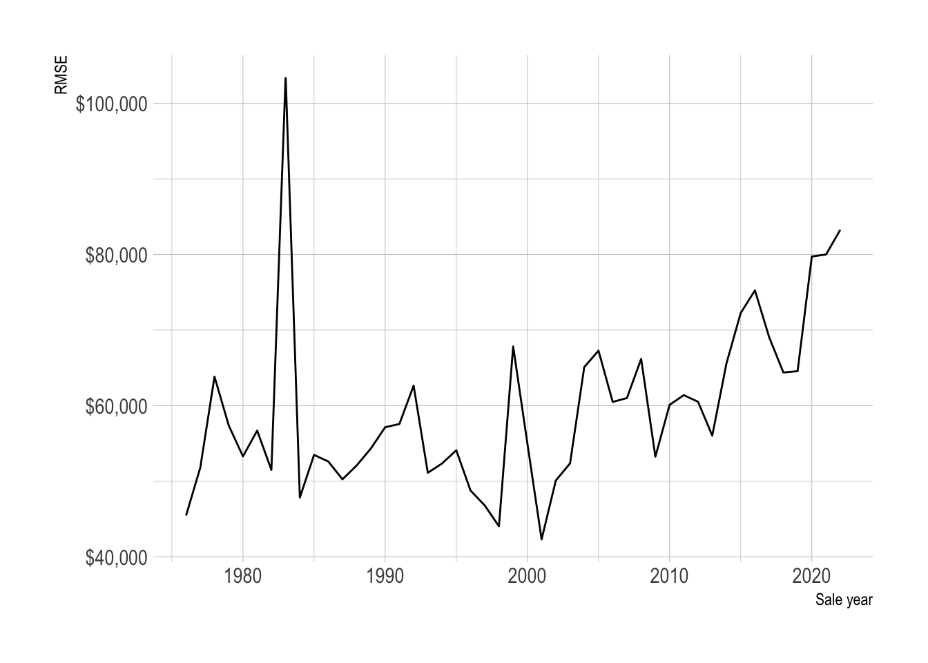
  group_by(sale_year) %>% 
  rmse(truth = sale_price_adj, estimate = .pred_dollar) %>% 
  ggplot(aes(sale_year, .estimate)) +
  geom_line() +
  scale_y_continuous(label = dollar) +
  labs(x = "Sale year",
       y = "RMSE")