Map Census Data With R

This talk was presented on May 30th, 2019 at Code For Pittsburgh.
Before we dive in, this presentation assumes that the user has basic familiarity with tidyverse, mainly dplyr. Knowing how to use %>% will be very helpful.
How to install packages:
install.packages("package_name")Get your census API key: https://api.census.gov/data/key_signup.html
Configure environment:
library(tidycensus)
library(tidyverse)
library(sf)
library(tigris)
library(ggmap)
library(janitor)

theme_set(theme_bw())

options(tigris_use_cache = TRUE,
        scipen = 4,
        digits = 3)
Packages
{tidycensus}
tidycensus gives access to the Census API and makes it easy to plot data on a map.
Data
- Demographics
- Decennial Census
- American Community Survey (ACS)
- error estimates
- Geometries
- country
- county
- zip code
- blocks
- tracts
- and more
{sf}
simple features makes it easy to work with polygon data in R. It uses the familiar tidyverse framework: everything is a tibble, and it uses %>%.
ggplot2::geom_sf() makes it easy to plot sf polygons.
sf can also do spatial calculations such as st_contains, st_intersects, and st_boundary.
{ggmap}
Uses Google Maps API to get basemaps. The API now requires a credit card, but it has a fairly generous “free” tier.
Using {tidycensus}
census_api_key("your_key_here")This loads the variables from the Decennial Census in 2010:
variables_dec <- load_variables(year = 2010, dataset = "sf1", cache = TRUE)## # A tibble: 3,346 x 3
## name label concept
## <chr> <chr> <chr>
## 1 H001001 Total HOUSING UNITS
## 2 H002001 Total URBAN AND RURAL
## 3 H002002 Total!!Urban URBAN AND RURAL
## 4 H002003 Total!!Urban!!Inside urbanized areas URBAN AND RURAL
## 5 H002004 Total!!Urban!!Inside urban clusters URBAN AND RURAL
## 6 H002005 Total!!Rural URBAN AND RURAL
## 7 H002006 Total!!Not defined for this file URBAN AND RURAL
## 8 H003001 Total OCCUPANCY STATUS
## 9 H003002 Total!!Occupied OCCUPANCY STATUS
## 10 H003003 Total!!Vacant OCCUPANCY STATUS
## # … with 3,336 more rowsThis loads the ACS variables for 2017:
variables_acs <- load_variables(year = 2017, dataset = "acs5", cache = TRUE)## # A tibble: 25,070 x 3
## name label concept
## <chr> <chr> <chr>
## 1 B00001_001 Estimate!!Total UNWEIGHTED SAMPLE COUNT OF THE PO…
## 2 B00002_001 Estimate!!Total UNWEIGHTED SAMPLE HOUSING UNITS
## 3 B01001_001 Estimate!!Total SEX BY AGE
## 4 B01001_002 Estimate!!Total!!Male SEX BY AGE
## 5 B01001_003 Estimate!!Total!!Male!!Under 5… SEX BY AGE
## 6 B01001_004 Estimate!!Total!!Male!!5 to 9 … SEX BY AGE
## 7 B01001_005 Estimate!!Total!!Male!!10 to 1… SEX BY AGE
## 8 B01001_006 Estimate!!Total!!Male!!15 to 1… SEX BY AGE
## 9 B01001_007 Estimate!!Total!!Male!!18 and … SEX BY AGE
## 10 B01001_008 Estimate!!Total!!Male!!20 years SEX BY AGE
## # … with 25,060 more rowsMap total population in the U.S.
Use View() to browse the variables
variables_dec %>%
  filter(str_detect(concept, "POPULATION")) %>%
  View()
P001001 has the data we are looking for.
Query the total population of the continental U.S. states:
states <- get_decennial(geography = "state",
                        variables = c(total_pop = "P001001"),
                        geometry = TRUE,
                        output = "wide")
The states tibble contains the census data and the polygons for the geometries.
## Simple feature collection with 52 features and 3 fields
## geometry type:  MULTIPOLYGON
## dimension:      XY
## bbox:           xmin: -179 ymin: 17.9 xmax: 180 ymax: 71.4
## geographic CRS: NAD83
## # A tibble: 52 x 4
##    GEOID NAME       total_pop                                           geometry
##    <chr> <chr>          <dbl>                                 <MULTIPOLYGON [°]>
##  1 23    Maine        1328361 (((-67.6 44.5, -67.6 44.5, -67.6 44.5, -67.6 44.5…
##  2 25    Massachus…   6547629 (((-70.8 41.6, -70.8 41.6, -70.8 41.6, -70.8 41.6…
##  3 26    Michigan     9883640 (((-88.7 48.1, -88.7 48.1, -88.7 48.1, -88.7 48.1…
##  4 30    Montana       989415 (((-104 45, -104 45, -104 45, -104 45, -105 45, -…
##  5 32    Nevada       2700551 (((-114 37, -114 37, -114 36.8, -114 36.7, -114 3…
##  6 34    New Jersey   8791894 (((-75.5 39.7, -75.5 39.7, -75.5 39.7, -75.5 39.7…
##  7 36    New York    19378102 (((-71.9 41.3, -71.9 41.3, -71.9 41.3, -71.9 41.3…
##  8 37    North Car…   9535483 (((-82.6 36, -82.6 36, -82.6 36, -82.6 36, -82.6 …
##  9 39    Ohio        11536504 (((-82.8 41.7, -82.8 41.7, -82.8 41.7, -82.8 41.7…
## 10 42    Pennsylva…  12702379 (((-75.4 39.8, -75.4 39.8, -75.5 39.8, -75.5 39.8…
## # … with 42 more rows
Make a bar graph with the data:
states %>%
  mutate(NAME = fct_reorder(NAME, total_pop)) %>%
  ggplot(aes(NAME, total_pop)) +
    geom_col() +
    coord_flip()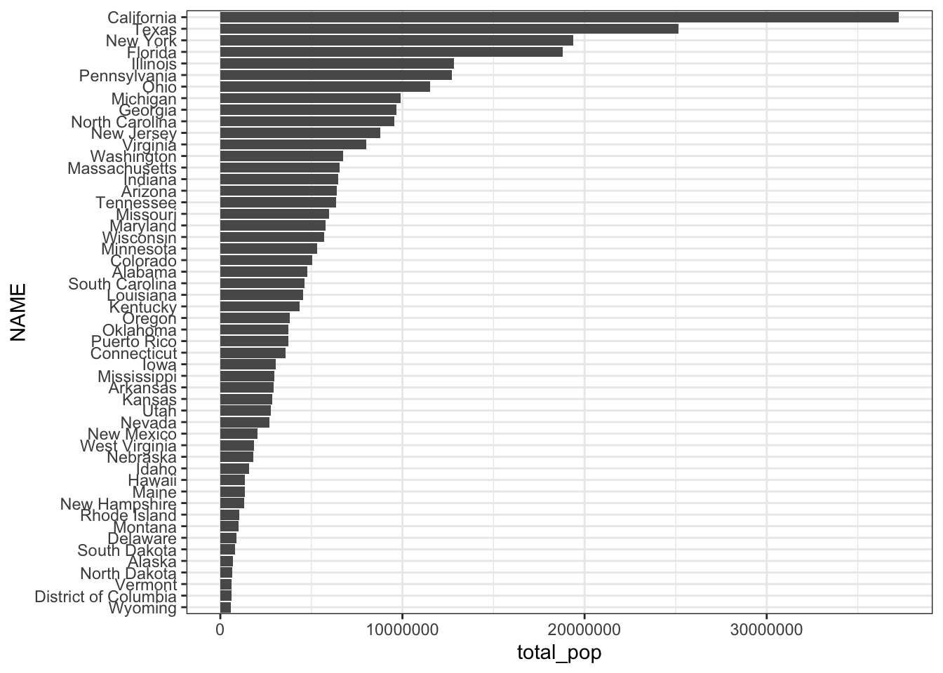
Plot the same data on a map:
states %>%
  filter(NAME != "Alaska",
         NAME != "Hawaii",
         !str_detect(NAME, "Puerto")) %>%
  ggplot(aes(fill = total_pop)) +
    geom_sf() +
    scale_fill_viridis_c("Total Population")
Pull the total population of each county in PA and plot it:
pennsylvania <- get_decennial(geography = "county",
                           variables = c(total_pop = "P001001"),
                           state = "PA",
                           geometry = TRUE,
                           output = "wide")
pennsylvania %>%
  ggplot(aes(fill = total_pop)) +
    geom_sf() +
    scale_fill_viridis_c()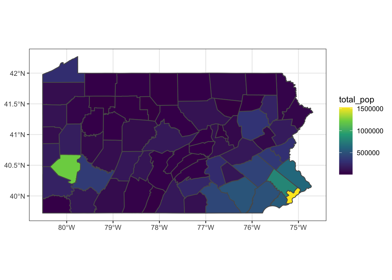
ggplot2 intelligently handles cases when we don’t have data for a certain polygon:
pennsylvania %>%
  mutate(total_pop = case_when(NAME == "Allegheny County, Pennsylvania" ~ NA_real_,
                               NAME != "Allegheny County, Pennsylvania" ~ total_pop)) %>%
  ggplot(aes(fill = total_pop)) +
    geom_sf() +
    scale_fill_viridis_c()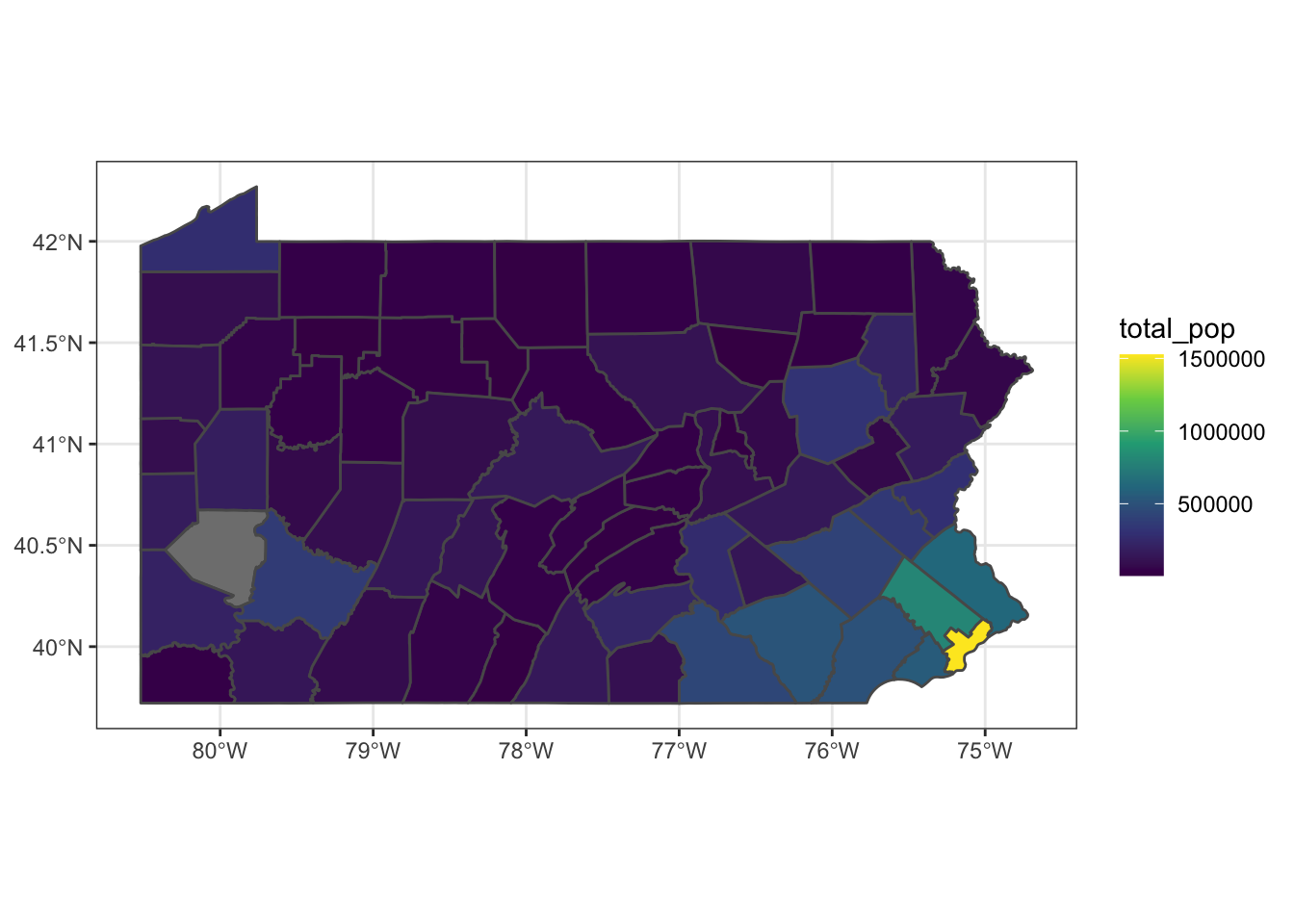
We can stack multiple polygons in the same graph to highlight Allegheny County:
allegheny <- pennsylvania %>%
  filter(str_detect(NAME, "Allegheny"))

pennsylvania %>%
  ggplot() +
    geom_sf(aes(fill = total_pop)) +
    geom_sf(data = allegheny, color = "white", linetype = 2, size = 1, alpha = 0) +
    scale_fill_viridis_c()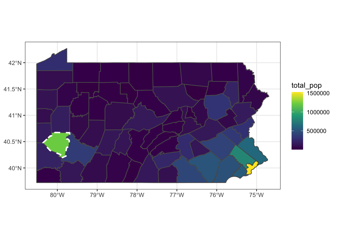
We can also use tidycensus to download demographic data for census tracts.
Set the variables we want to use first:
racevars <- c(White = "P005003",
              Black = "P005004",
              Asian = "P005006",
              Hispanic = "P004003")
#note that this data is long, not wide
allegheny_tracts <- get_decennial(geography = "tract", variables = racevars,
                        state = "PA", county = "Allegheny County", geometry = TRUE,
                        summary_var = "P001001")
Calculate as a percentage of tract population:
allegheny_tracts <- allegheny_tracts %>%
  mutate(pct = 100 * value / summary_value)
Facet by variable and map the data:
allegheny_tracts %>%
  ggplot(aes(fill = pct)) +
    geom_sf(color = NA) +
    facet_wrap(~variable) +
    scale_fill_viridis_c()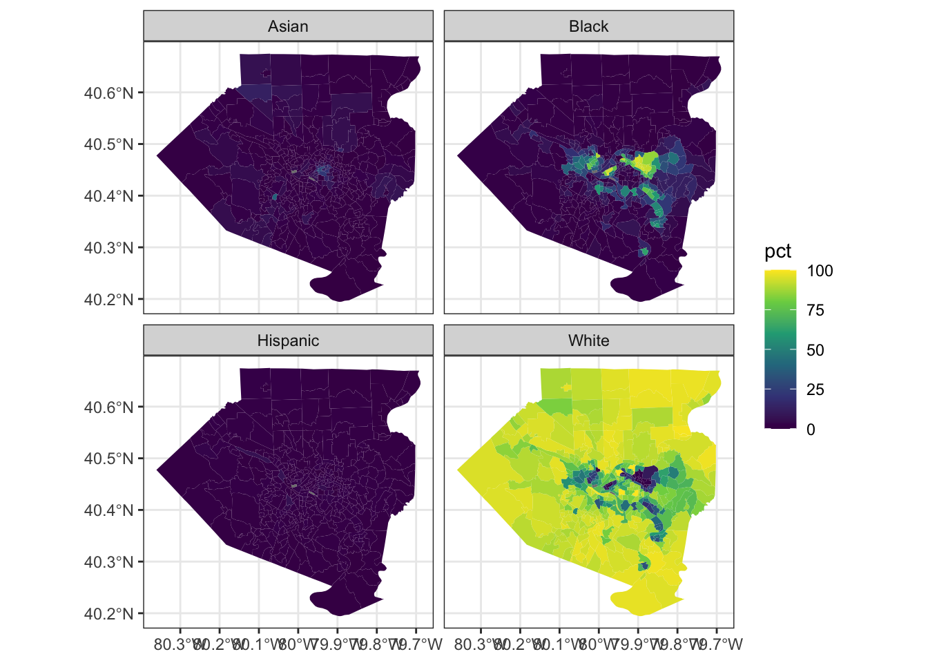
We can overlay the boundaries of Pittsburgh over the same graph.
Download the boundary shapefile and use sf::st_read to read it into R:
city_pgh <- st_read("data/Pittsburgh_City_Boundary-shp/City_Boundary.shp")## Reading layer `City_Boundary' from data source `/Users/conortompkins/github_repos/blog_hugo_academic/content/post/map-census-data-with-r/data/Pittsburgh_City_Boundary-shp/City_Boundary.shp' using driver `ESRI Shapefile'
## Simple feature collection with 8 features and 8 fields
## geometry type: POLYGON
## dimension: XY
## bbox: xmin: -80.1 ymin: 40.4 xmax: -79.9 ymax: 40.5
## geographic CRS: WGS 84allegheny_tracts %>%
ggplot() +
geom_sf(aes(fill = pct), color = NA) +
geom_sf(data = city_pgh, color = "white", linetype = 2, size = 1, alpha = 0) +
facet_wrap(~variable) +
scale_fill_viridis_c()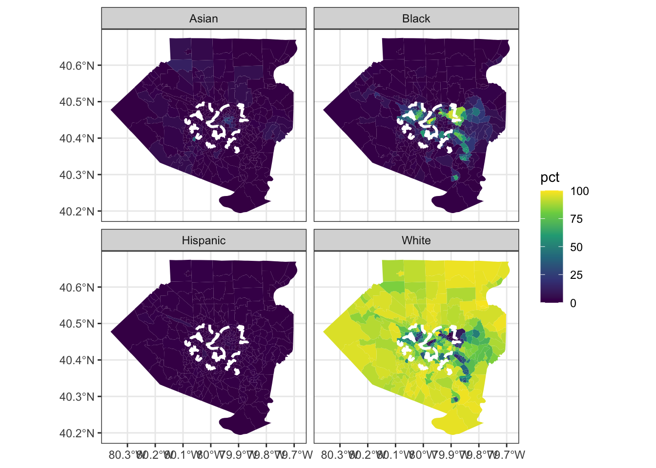
Working with other data
WPRDC 311 data and city wards
We can also download the shapefile for the City of Pittsburgh wards. The 311 dataset is tagged with the ward the request originated from, so we can use that to aggregate and map the total number of 311 requests per ward.
df_311 <- read_csv("https://data.wprdc.org/datastore/dump/76fda9d0-69be-4dd5-8108-0de7907fc5a4") %>%
clean_names()| request_id | created_on | request_type | request_origin | status | department | neighborhood | council_district | ward |
|---|---|---|---|---|---|---|---|---|
| 203364 | 2017-12-15 14:53:00 | Street Obstruction/Closure | Call Center | 1 | DOMI - Permits | Central Northside | 1 | 22 |
| 200800 | 2017-11-29 09:54:00 | Graffiti | Control Panel | 1 | Police - Zones 1-6 | South Side Flats | 3 | 16 |
| 201310 | 2017-12-01 13:23:00 | Litter | Call Center | 1 | DPW - Street Maintenance | Troy Hill | 1 | 24 |
| 200171 | 2017-11-22 14:54:00 | Water Main Break | Call Center | 1 | Pittsburgh Water and Sewer Authority | Banksville | 2 | 20 |
| 193043 | 2017-10-12 12:46:00 | Guide Rail | Call Center | 1 | DPW - Construction Division | East Hills | 9 | 13 |
| 196521 | 2017-10-31 15:17:00 | Guide Rail | Call Center | 1 | DPW - Construction Division | East Hills | 9 | 13 |
| 193206 | 2017-10-13 09:18:00 | Sidewalk/Curb/HC Ramp Maintenance | Call Center | 1 | DOMI - Permits | Mount Washington | 4 | 19 |
| 195917 | 2017-10-27 10:23:00 | Manhole Cover | Call Center | 1 | DOMI - Permits | Bluff | 6 | 1 |
| 179176 | 2017-08-14 14:00:00 | Neighborhood Issues | Control Panel | 0 | NA | Middle Hill | 6 | 5 |
| 190422 | 2017-09-29 11:46:00 | Mayor’s Office | Website | 1 | 311 | North Oakland | 8 | 4 |
## Simple feature collection with 35 features and 7 fields
## geometry type:  POLYGON
## dimension:      XY
## bbox:           xmin: -80.1 ymin: 40.4 xmax: -79.9 ymax: 40.5
## geographic CRS: WGS 84
## First 10 features:
##    fid wards wards_id ward wardtext shape_leng shape_area
## 1    2     3        0   19       19     0.2389  0.0011446
## 2    3     4        0   24       24     0.0734  0.0001901
## 3    4     5        0   24       24     0.0274  0.0000210
## 4    5     6        0   20       20     0.2888  0.0011755
## 5    6     7        0   21       21     0.0619  0.0002074
## 6    7     8        0   23       23     0.0480  0.0001031
## 7    8     9        0   22       22     0.0593  0.0001967
## 8    9    10        0   26       26     0.1915  0.0009079
## 9   10    11        0   27       27     0.1173  0.0005849
## 10  11    12        0   27       27     0.0400  0.0000634
##                          geometry
## 1  POLYGON ((-80 40.4, -80 40....
## 2  POLYGON ((-80 40.5, -80 40....
## 3  POLYGON ((-80 40.5, -80 40....
## 4  POLYGON ((-80 40.4, -80 40....
## 5  POLYGON ((-80 40.5, -80 40....
## 6  POLYGON ((-80 40.5, -80 40....
## 7  POLYGON ((-80 40.5, -80 40....
## 8  POLYGON ((-80 40.5, -80 40....
## 9  POLYGON ((-80 40.5, -80 40....
## 10 POLYGON ((-80 40.5, -80 40....
Plot the ward polygons:
wards %>%
  ggplot() +
  geom_sf()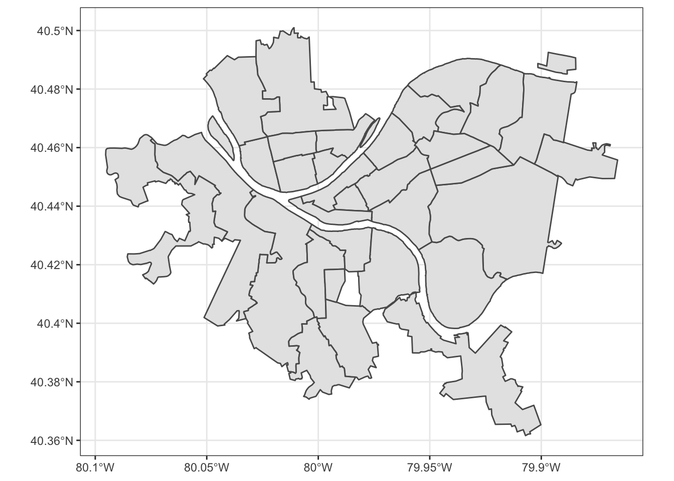
Calculate the center of each ward. We will use this to label the wards on the map:
ward_labels <- wards %>%
  st_centroid() %>%
  st_coordinates() %>%
  as_tibble() %>%
clean_names()| x | y |
|---|---|
| -80 | 40.4 |
| -80 | 40.5 |
| -80 | 40.5 |
| -80 | 40.4 |
| -80 | 40.5 |
Count the number of requests per ward:
df_311_count <- df_311 %>%
  count(ward, sort = TRUE)
Use left_join and bind_cols to join the count data with the coordinates:
ward_311 <- wards %>%
  left_join(df_311_count) %>%
  bind_cols(ward_labels)
## Simple feature collection with 35 features and 10 fields
## geometry type: POLYGON
## dimension: XY
## bbox: xmin: -80.1 ymin: 40.4 xmax: -79.9 ymax: 40.5
## geographic CRS: WGS 84
## First 10 features:
## fid wards wards_id ward wardtext shape_leng shape_area n x y
## 1 2 3 0 19 19 0.2389 0.0011446 35823 -80 40.4
## 2 3 4 0 24 24 0.0734 0.0001901 7049 -80 40.5
## 3 4 5 0 24 24 0.0274 0.0000210 7049 -80 40.5
## 4 5 6 0 20 20 0.2888 0.0011755 22617 -80 40.4
## 5 6 7 0 21 21 0.0619 0.0002074 5120 -80 40.5
## 6 7 8 0 23 23 0.0480 0.0001031 6394 -80 40.5
## 7 8 9 0 22 22 0.0593 0.0001967 6043 -80 40.5
## 8 9 10 0 26 26 0.1915 0.0009079 15065 -80 40.5
## 9 10 11 0 27 27 0.1173 0.0005849 14013 -80 40.5
## 10 11 12 0 27 27 0.0400 0.0000634 14013 -80 40.5
## geometry
## 1 POLYGON ((-80 40.4, -80 40....
## 2 POLYGON ((-80 40.5, -80 40....
## 3 POLYGON ((-80 40.5, -80 40....
## 4 POLYGON ((-80 40.4, -80 40....
## 5 POLYGON ((-80 40.5, -80 40....
## 6 POLYGON ((-80 40.5, -80 40....
## 7 POLYGON ((-80 40.5, -80 40....
## 8 POLYGON ((-80 40.5, -80 40....
## 9 POLYGON ((-80 40.5, -80 40....
## 10 POLYGON ((-80 40.5, -80 40....Plot the data:
ward_311 %>%
  ggplot() +
    geom_sf(aes(fill = n), color = NA) +
    geom_label(aes(x, y, label = ward), size = 3) +
    scale_fill_viridis_c("Number of 311 requests")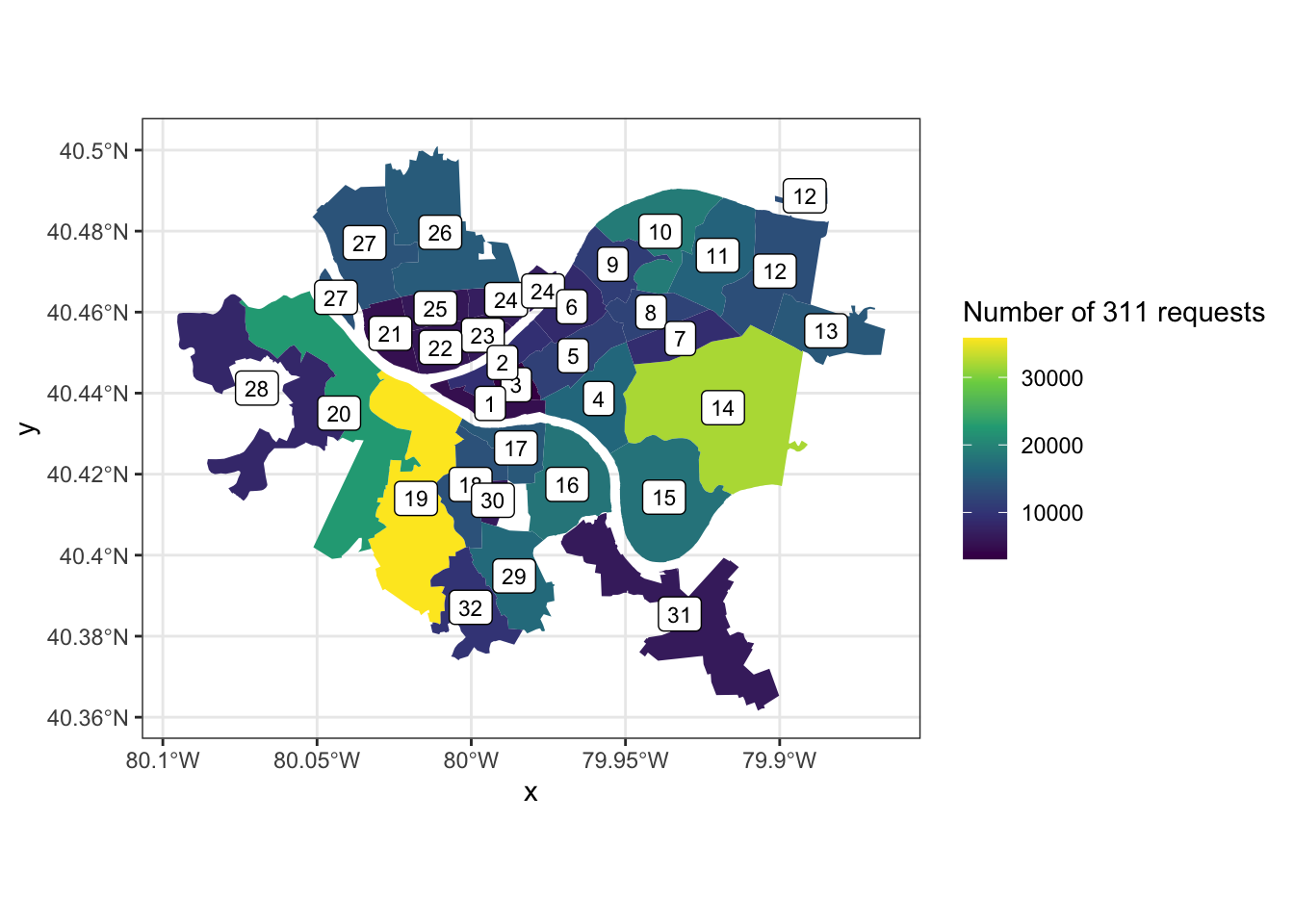
WPRDC overdose data
We can use the census data to adjust other data for per capita rates. For example, the WPRDC’s overdose data has the zip code that the overdose occurred in.
First, download the overdose dataset and pull the population data for each zip code:
df_overdose <- read_csv("https://data.wprdc.org/datastore/dump/1c59b26a-1684-4bfb-92f7-205b947530cf") %>%
  clean_names() %>%
  mutate(incident_zip = str_sub(incident_zip, 1, 5))

all_zips <- get_acs(geography = "zip code tabulation area",
                    variables = c(total_pop = "B01003_001"),
                    geometry = TRUE,
                    output = "wide")
Then, aggregate the overdose data to the zip code and join the datasets:
df_overdose <- df_overdose %>%
  count(incident_zip, sort = TRUE)

attempt1 <- all_zips %>%
  semi_join(df_overdose, by = c("GEOID" = "incident_zip")) %>%
  left_join(df_overdose, by = c("GEOID" = "incident_zip"))

attempt1 %>%
  ggplot() +
    geom_sf()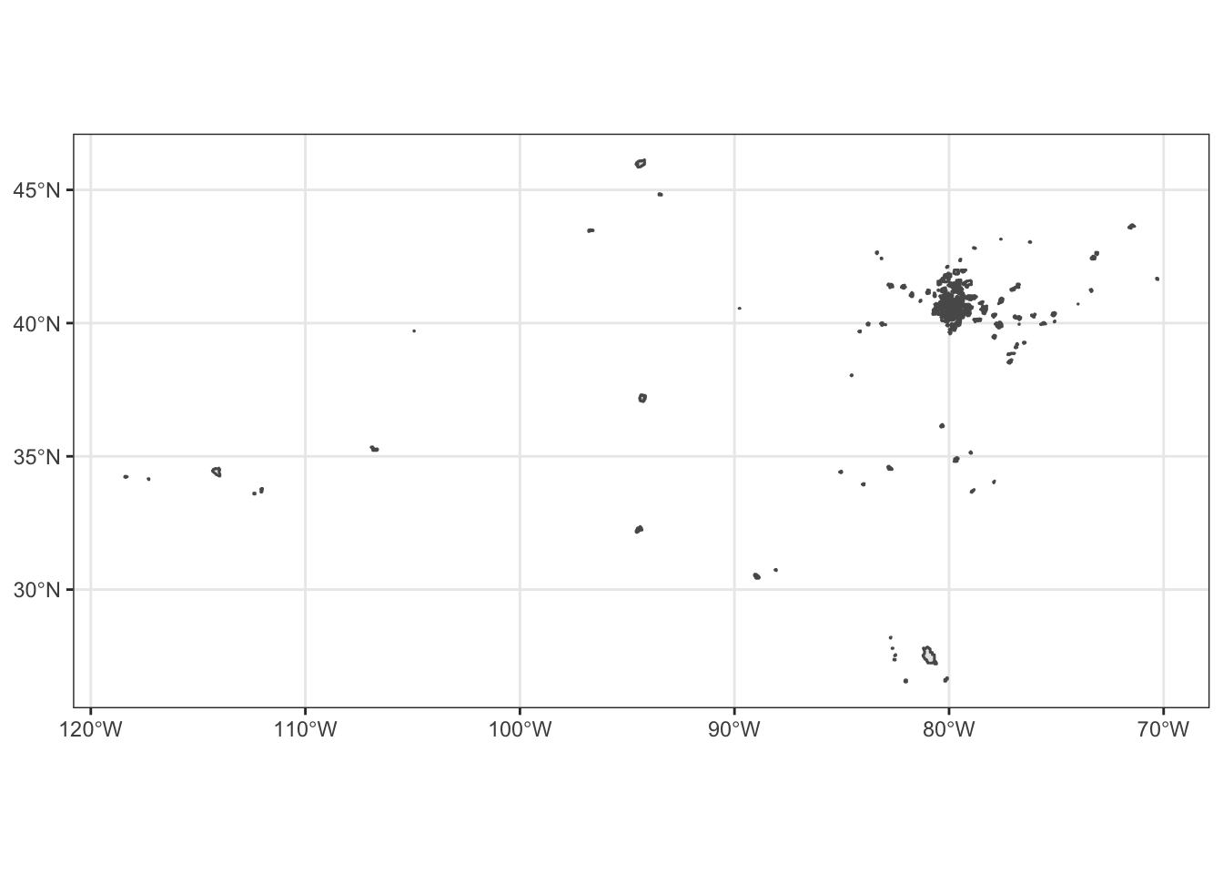
Unfortunately the data is kind of messy and includes zip codes that aren’t in Allegheny County.
We can use st_intersection to exclude all of the zip code polygons that do not fall within the allegheny county tibble we made earlier:
allegheny %>%
  ggplot() +
    geom_sf()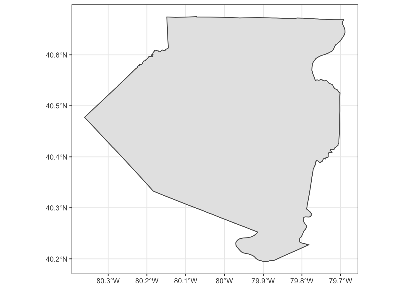
Then, join the aggregated overdose data with left_join:
df_allegheny_overdose <- st_intersection(allegheny, all_zips) %>%
  left_join(df_overdose, by = c("GEOID.1" = "incident_zip"))
Now we can calculate the per 1,000 overdose rate and plot the data:
df_allegheny_overdose %>%
  filter(total_popE >= 400) %>%
  mutate(overdoses_per_capita = n / total_popE * 1000) %>%
  ggplot(aes(fill = overdoses_per_capita)) +
    geom_sf(color = NA) +
    scale_fill_viridis_c()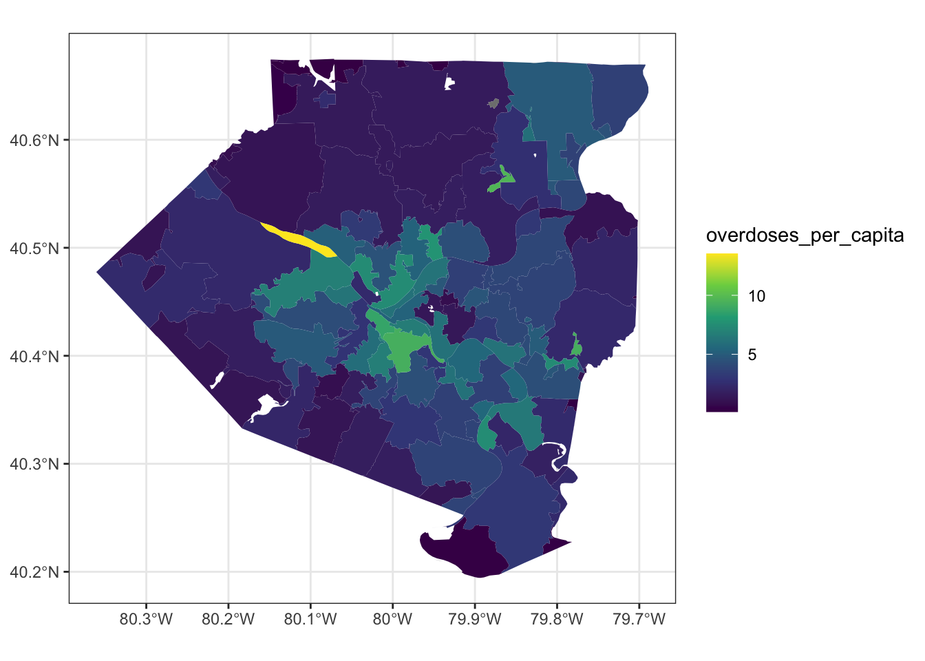
{ggmap} basemaps
We can use ggmap to request a basemap from the Google Maps API.
Get your API key here
register_google(key = "Your key here")pgh_map <- get_map(location = c(lat = 40.445315, lon = -79.977104), zoom = 12)
ggmap(pgh_map)
There are multiple basemap styles available:
get_map(location = c(lat = 40.445315, lon = -79.977104), zoom = 12, maptype = "satellite", source = "google") %>%
  ggmap()
get_map(location = c(lat = 40.445315, lon = -79.977104), zoom = 12, maptype = "roadmap", source = "google") %>%
  ggmap()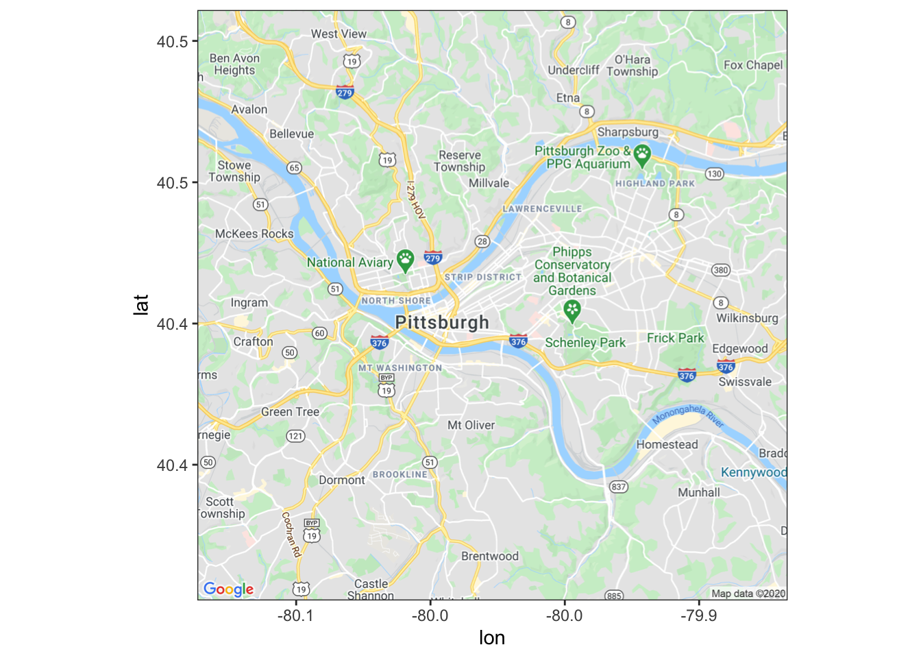
get_map(location = c(lat = 40.445315, lon = -79.977104), zoom = 12, maptype = "watercolor", source = "google") %>%
  ggmap()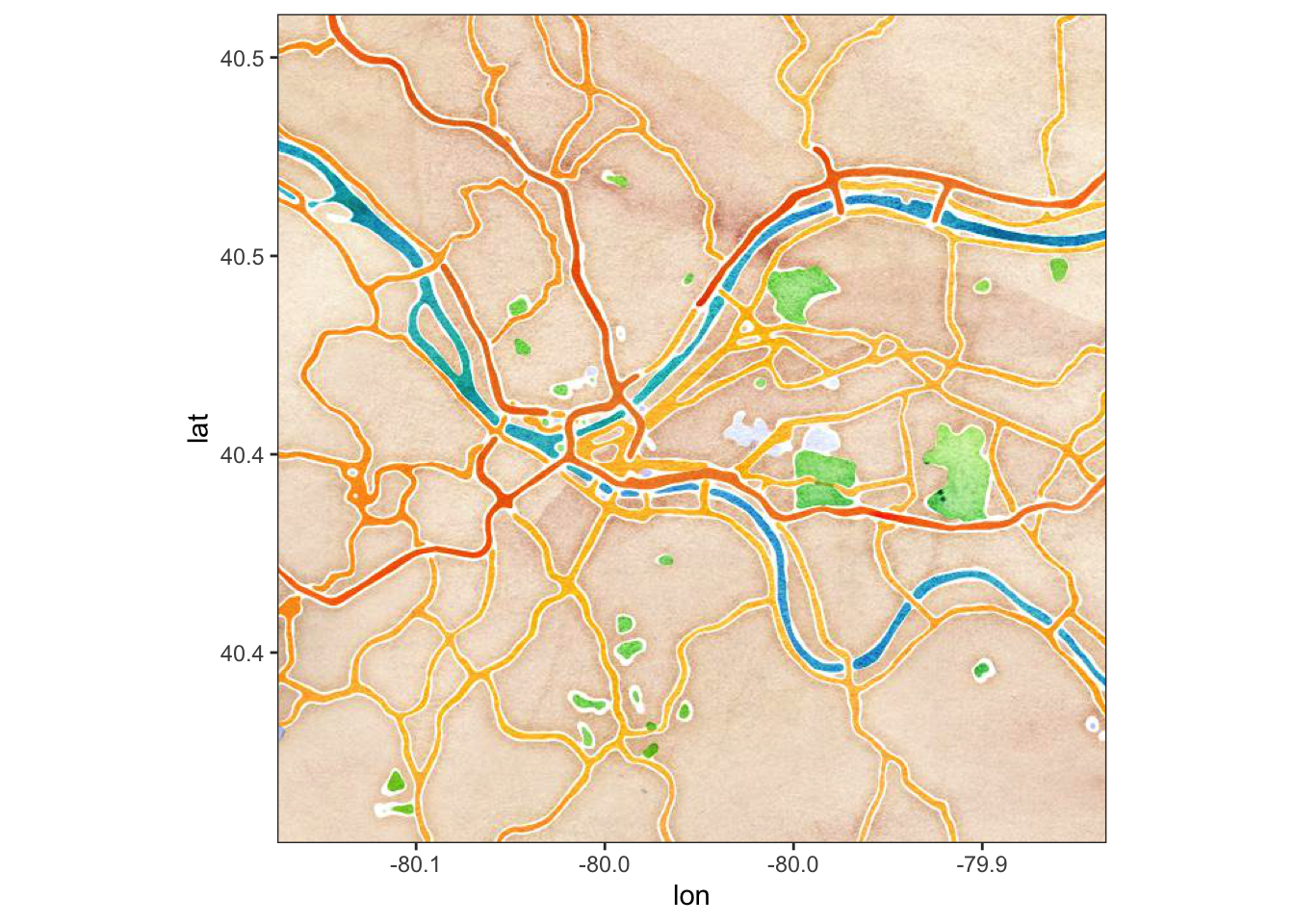
get_map(location = c(lat = 40.445315, lon = -79.977104), zoom = 12, maptype = "toner", source = "stamen") %>%
  ggmap()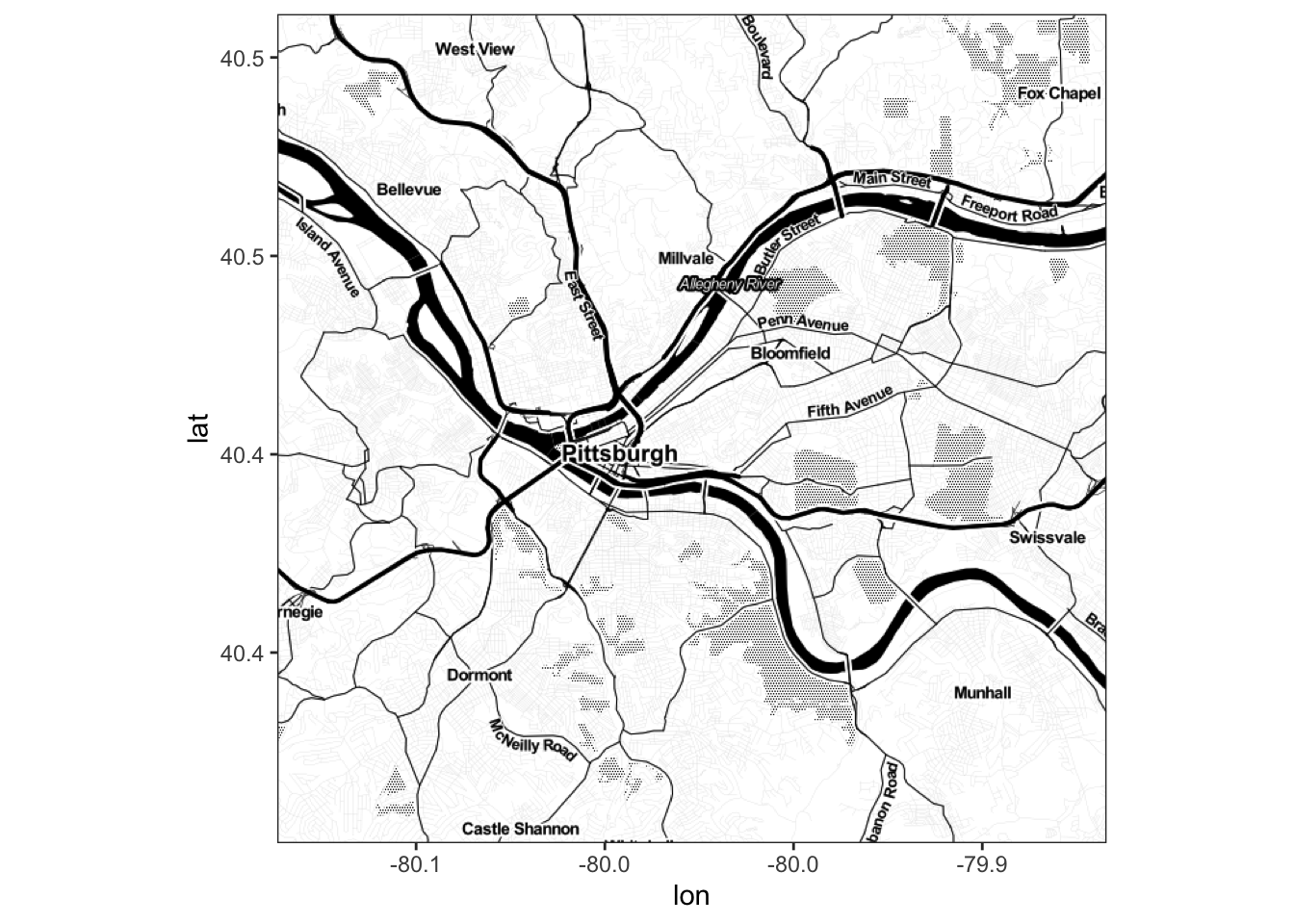
Combining maps from different systems requires us to use the same map projection. Google uses 4326. Use coord_sf to set the projection:
ggmap(pgh_map) +
  geom_sf(data = ward_311, aes(fill = n), inherit.aes = FALSE, color = NA, alpha = .7) +
  geom_label(data = ward_311, aes(x, y, label = ward), size = 3) +
  coord_sf(crs = st_crs(4326)) +
  scale_fill_viridis_c("Number of 311 requests")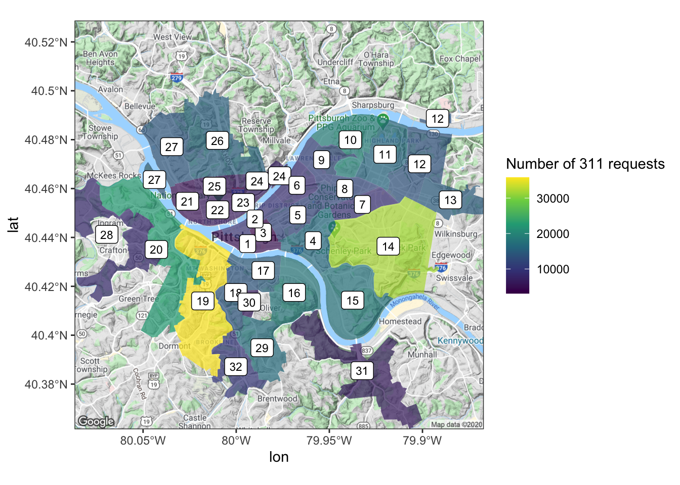
Links
- https://walkerke.github.io/tidycensus/articles/basic-usage.html
- https://walkerke.github.io/tidycensus/reference/get_acs.html
- https://walkerke.github.io/tidycensus/articles/spatial-data.html
- https://walkerke.github.io/tidycensus/articles/other-datasets.html
- https://cengel.github.io/R-spatial/mapping.html
- https://www.r-spatial.org/r/2018/10/25/ggplot2-sf.html
- https://www.r-spatial.org/r/2018/10/25/ggplot2-sf-2.html
- https://www.r-spatial.org/r/2018/10/25/ggplot2-sf-3.html
- google maps API key: https://cloud.google.com/maps-platform/
- https://lucidmanager.org/geocoding-with-ggmap/
- https://github.com/rstudio/cheatsheets/blob/master/sf.pdf