Training set metrics (75% of total observations)

I used 10-fold cross-validation to assess model performance against the training set:

train_metrics %>% 
  select(model_name, id, .metric, .estimate) %>% 
  pivot_wider(names_from = .metric, values_from = .estimate) %>% 
  ggplot(aes(rmse, rsq, color = model_name)) +
  geom_point() +
  scale_x_continuous(label = dollar) +
  labs(x = "Root Mean Squared Error",
       y = "R^2")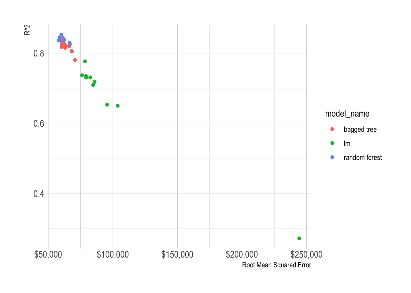

Test set metrics (25% of total observations)

test_metrics %>% 
  select(.metric, .estimate)

## # A tibble: 3 x 2
##   .metric   .estimate
##   <chr>         <dbl>
## 1 rmse     216212.   
## 2 rsq           0.628
## 3 mape    3229245.

model_results %>% 
  ggplot(aes(.resid)) +
  geom_density() +
  geom_vline(xintercept = 0, lty = 2) +
  scale_x_continuous(label = label_dollar())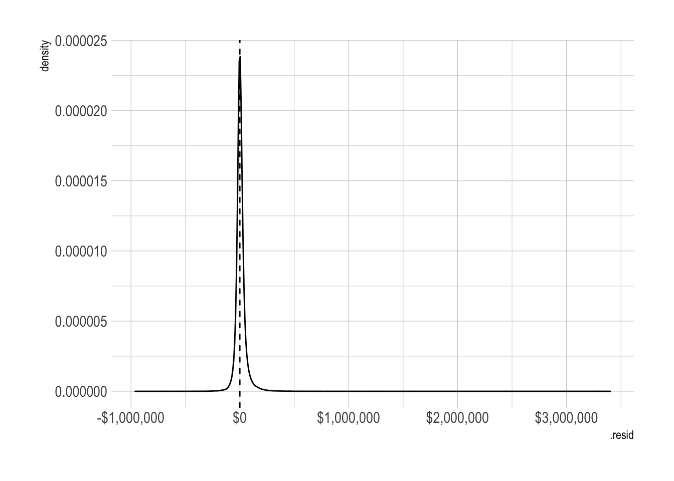

model_results %>% 
  ggplot(aes(sale_price_adj, .pred_dollar)) +
  geom_density_2d_filled(contour_var = "count") +
  scale_x_log10(label = label_dollar()) +
  scale_y_log10(label = label_dollar()) +
  guides(fill = guide_coloursteps()) +
  labs(x = "Inflation-adjusted sale price log10 scale",
       y = "Prediction",
       fill = "Sales")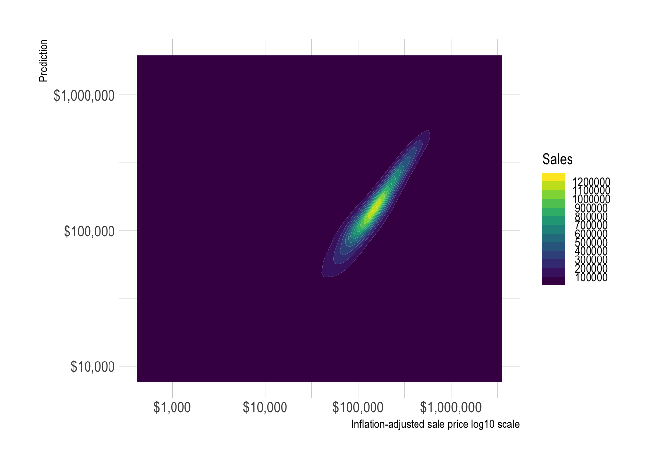

The model becomes less effective as the actual sale price increases.

model_results %>% 
  ggplot(aes(sale_price_adj, .resid)) +
  geom_point(alpha = .01) +
  scale_x_log10(label = dollar) +
  scale_y_continuous(label = dollar) +
  labs(x = "Inflation-adjusted sale price log10 scale",
       y = "Residual")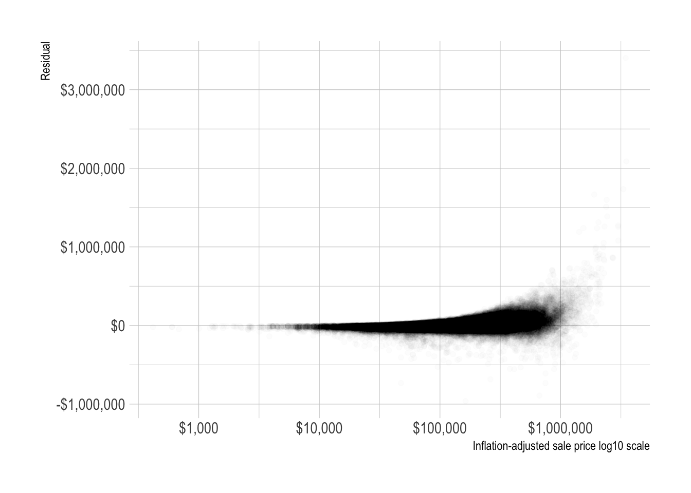

geo_ids <- st_read("data/unified_geo_ids/unified_geo_ids.shp",
                   quiet = T)

geo_id_median_resid <- model_results %>% 
  group_by(geo_id) %>% 
  summarize(median_resid = median(.resid))

pal <- colorNumeric(
  palette = "viridis",
  domain = geo_id_median_resid$median_resid)

leaflet_map <- geo_ids %>% 
  left_join(geo_id_median_resid) %>% 
  leaflet() %>% 
  addProviderTiles(providers$Stamen.TonerLite,
                   options = providerTileOptions(noWrap = TRUE,
                                                 minZoom = 9, 
                                                 #maxZoom = 8
                   )) %>% 
  addPolygons(popup = ~ str_c(geo_id, " ", "median residual: ", round(median_resid, 2), sep = ""),
              fillColor = ~pal(median_resid),
              fillOpacity = .7,
              color = "black",
              weight = 3) %>% 
  addLegend("bottomright", pal = pal, values = ~median_resid,
            title = "Median of residual",
            opacity = 1)

widgetframe::frameWidget(leaflet_map)

model_results %>% 
  add_count(geo_id) %>% 
  mutate(geo_id = fct_reorder(geo_id, .resid, .fun = median)) %>% 
  ggplot(aes(.resid, geo_id, fill = n)) +
  geom_boxplot(color = "grey",
               outlier.alpha = 0) +
  geom_vline(xintercept = 0, lty = 2, color = "red") +
  scale_fill_viridis_c() +
  coord_cartesian(xlim = c(-10^5, 10^5)) +
  labs(fill = "Sales")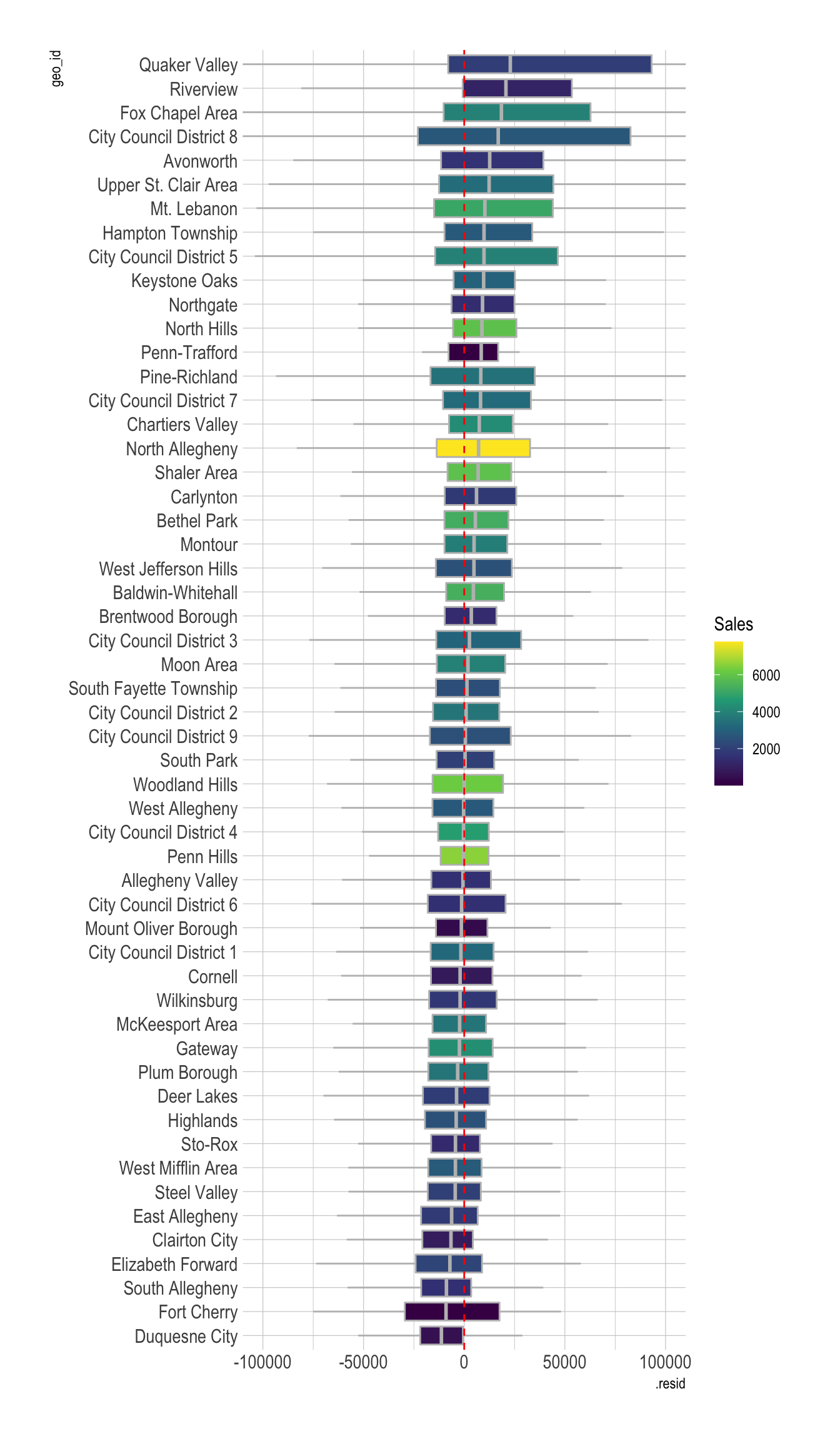

model_results %>% 
  add_count(style_desc) %>% 
  mutate(style_desc = fct_reorder(style_desc, .resid, .fun = median)) %>% 
  ggplot(aes(.resid, style_desc, fill = n)) +
  geom_boxplot(color = "grey",
               outlier.alpha = 0) +
  geom_vline(xintercept = 0, lty = 2, color = "red") +
  coord_cartesian(xlim = c(-10.5^5, 10.5^5)) +
  scale_x_continuous(labels = label_dollar()) +
  scale_fill_viridis_c() +
  labs(fill = "Sales",
       x = "Residual",
       y = "House style")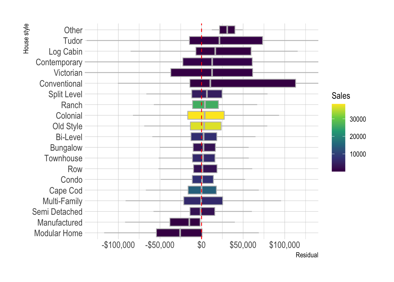

model_results %>% 
  add_count(grade_desc) %>% 
  mutate(grade_desc = fct_reorder(grade_desc, .resid, .fun = median)) %>% 
  ggplot(aes(.resid, grade_desc, fill = n)) +
  geom_boxplot(color = "grey",
               outlier.alpha = 0) +
  scale_fill_viridis_c() +
  scale_x_continuous(labels = label_dollar()) +
  coord_cartesian(xlim = c(-10^5, 10.5^6)) +
  labs(x = "Residual",
       y = "Grade",
       fill = "Sales")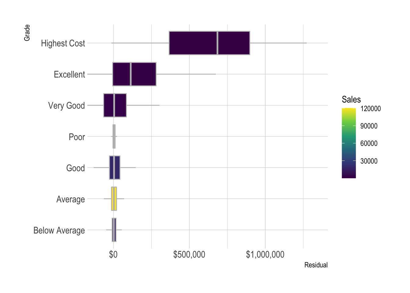

model_results %>% 
  add_count(condition_desc) %>% 
  mutate(condition_desc = fct_explicit_na(condition_desc),
         condition_desc = fct_reorder(condition_desc, .resid, .fun = median)) %>% 
  ggplot(aes(.resid, condition_desc, fill = n)) +
  geom_boxplot(color = "grey",
               outlier.alpha = 0) +
  geom_vline(xintercept = 0, lty = 2, color = "red") +
  scale_fill_viridis_c() +
  scale_x_continuous(labels = label_dollar()) +
  coord_cartesian(xlim = c(-10^5, 10.5^5)) +
  labs(x = "Residual",
       y = "Condition",
       fill = "Sales")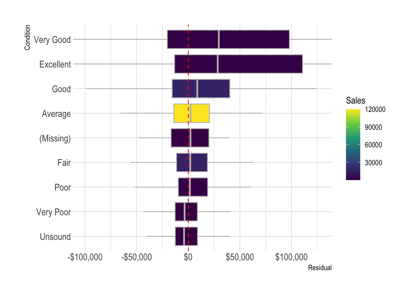

model_results %>% 
  ggplot(aes(finished_living_area, .resid)) +
  geom_point(alpha = .1) +
  scale_x_log10() +
  scale_y_continuous(label = dollar) +
  labs(x = "Finished Living Area sq. ft. log10 scale",
       y = "Residual")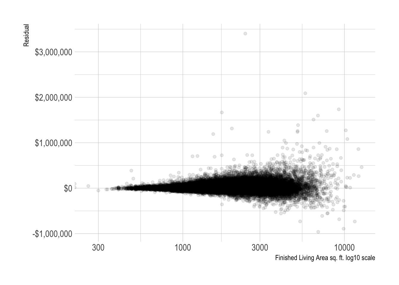

model_results %>% 
  ggplot(aes(lot_area, .resid)) +
  geom_point(alpha = .1) +
  scale_x_log10(labels = label_comma()) +
  scale_y_continuous(labels = label_dollar()) +
  labs(x = "Lot Area sq. ft. log10 scale",
       y = "Residual")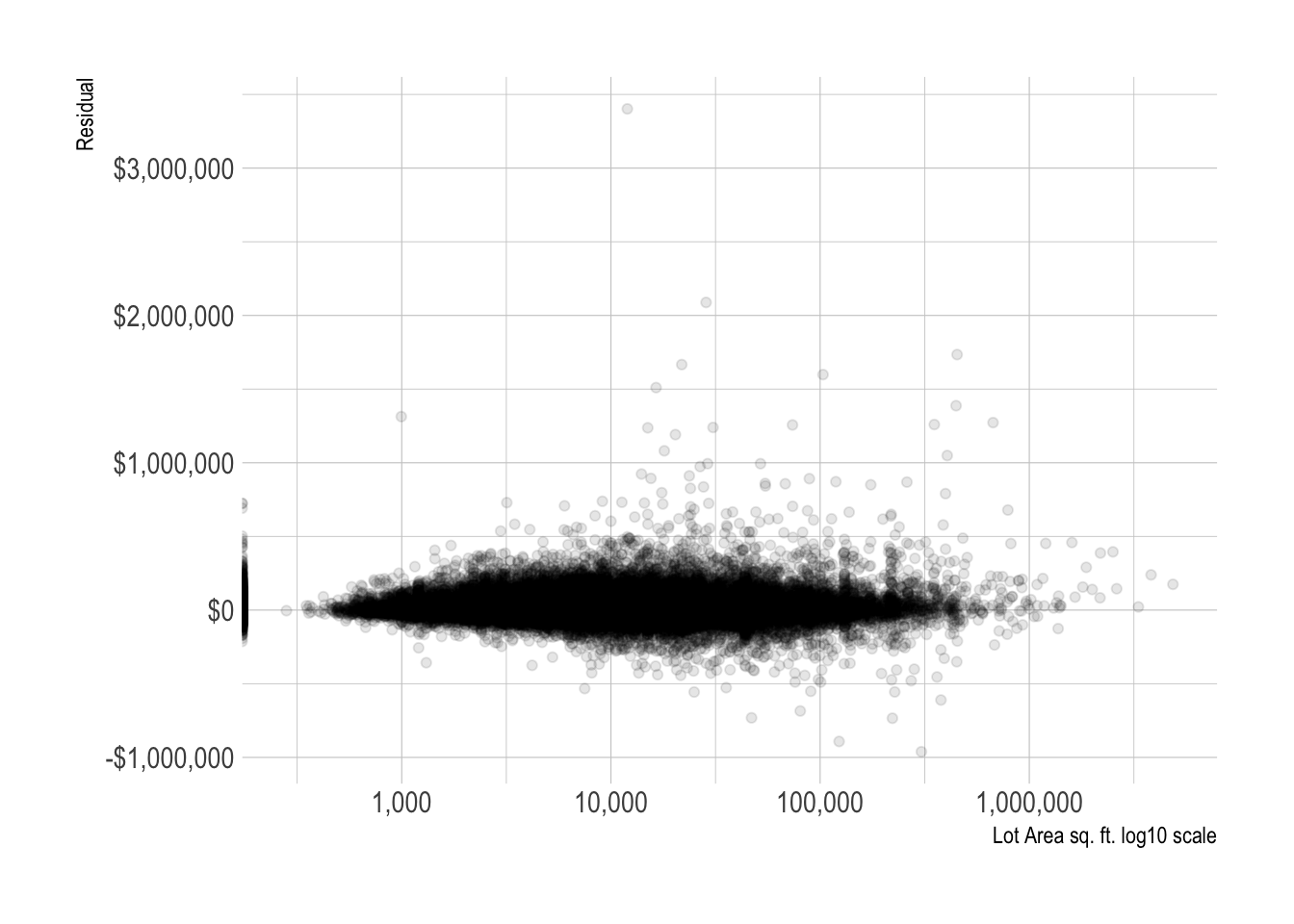

model_results %>% 
  group_by(house_age_at_sale) %>% 
  rmse(truth = sale_price_adj, estimate = .pred_dollar) %>% 
  ggplot(aes(house_age_at_sale, .estimate)) +
  geom_point(alpha = .5) +
  scale_y_continuous(labels = label_dollar()) +
  labs(x = "House age at sale",
       y = "RMSE")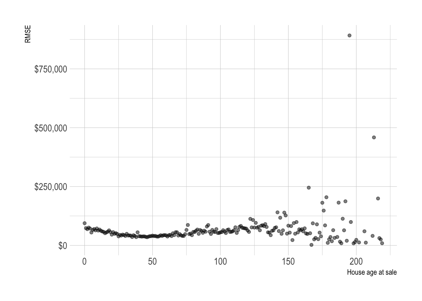

The model is best at predicting the sale price of houses built in the 1940s to 1980s. This is when most of the houses in the county were built.

model_results %>% 
  group_by(year_built) %>% 
  rmse(truth = sale_price_adj, estimate = .pred_dollar) %>% 
  ggplot(aes(year_built, .estimate)) +
  geom_point(alpha = .5) +
  scale_y_continuous(labels = label_dollar()) +
  labs(x = "Year Built",
       y = "RMSE")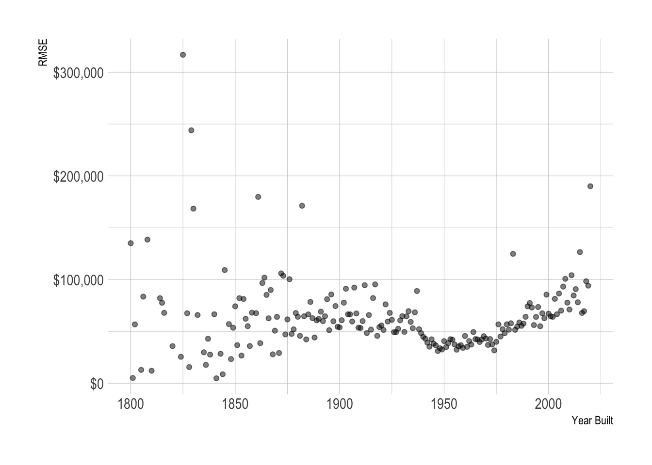

model_results %>% 
  add_count(bedrooms) %>% 
  ggplot(aes(.resid, bedrooms, group = bedrooms, fill = n)) +
  geom_boxplot(color = "grey",
               outlier.alpha = 0) +
  geom_vline(xintercept = 0, lty = 2, color = "red") +
  scale_y_continuous(breaks = c(0:15)) +
  scale_fill_viridis_c() +
  scale_x_continuous(labels = label_dollar()) +
  coord_cartesian(xlim = c(-10^5, 10^5)) +
  labs(x = "Residual",
       y = "Bedrooms",
       fill = "Sales")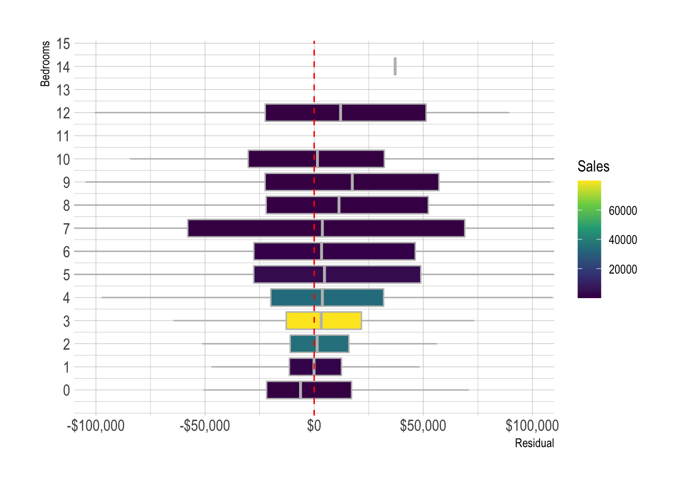

model_results %>% 
  add_count(full_baths) %>% 
  ggplot(aes(.resid, full_baths, group = full_baths, fill = n)) +
  geom_boxplot(color = "grey",
               outlier.alpha = 0) +
  geom_vline(xintercept = 0, lty = 2, color = "red") +
  scale_y_continuous(breaks = c(0:12)) +
  scale_fill_viridis_c() +
  scale_x_continuous(label = dollar) +
  coord_cartesian(xlim = c(-10^5, 750000)) +
  labs(x = "Residual",
       y = "Full bathrooms",
       fill = "Sales")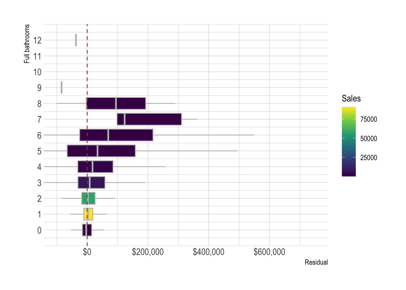

model_results %>% 
  add_count(half_baths) %>% 
  ggplot(aes(.resid, half_baths, group = half_baths, fill = n)) +
  geom_boxplot(color = "grey",
               outlier.alpha = 0) +
  geom_vline(xintercept = 0, lty = 2, color = "red") +
  scale_y_continuous(breaks = c(0:8)) +
  scale_x_continuous(labels = label_dollar()) +
  scale_fill_viridis_c() +
  coord_cartesian(xlim = c(-10^5, 10^5)) +
  labs(x = "Residual",
       y = "Half bathrooms",
       fill = "Sales")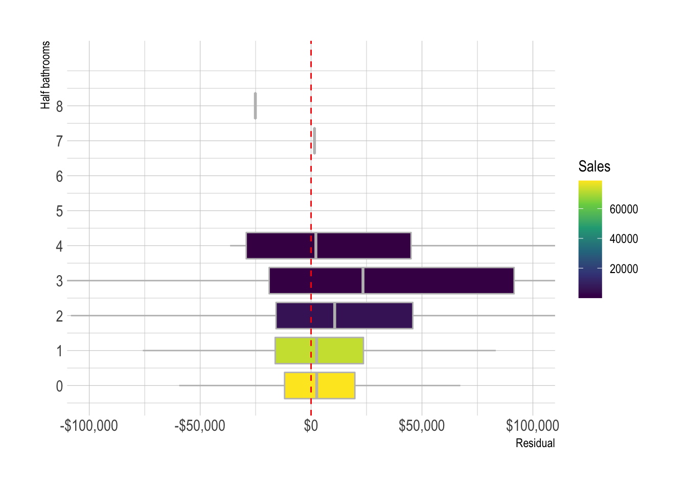

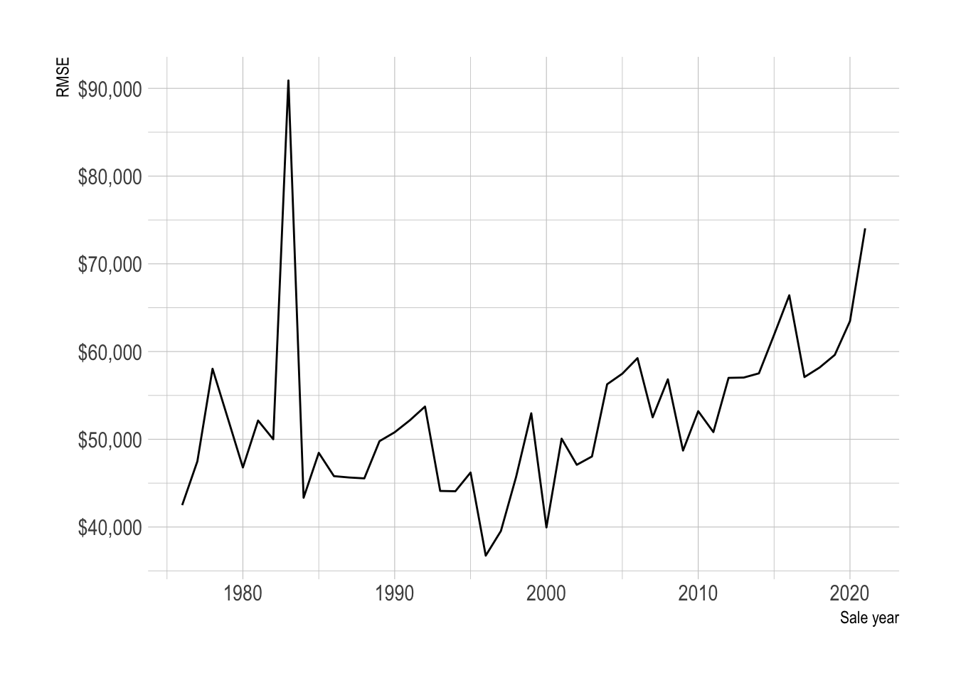
model_results %>% 
  group_by(sale_year) %>% 
  rmse(truth = sale_price_adj, estimate = .pred_dollar) %>% 
  ggplot(aes(sale_year, .estimate)) +
  geom_line() +
  scale_y_continuous(label = dollar) +
  labs(x = "Sale year",
       y = "RMSE")